Types of Portfolio Average Returns

OK so today’s topic — holding period return, or HPR.

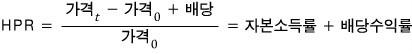
(For bonds, swap “dividends” for “interest payments” and you’re good.)

But notice — that formula up there is looking at the whole holding period at once. So sure, it computes cleanly enough, and you can convert it to an annual rate, no problem.

The trouble shows up when returns pile on top of each other over several years. At that point it gets genuinely ambiguous how you should average all those returns into one number.

So the move is basically: list out a few flavors of average and pick whichever one fits the situation. That kinda thing.

Let’s run through them.

Arithmetic Average Return

The arithmetic average is just… the average. The one we use for everything in normal life!!!

The class’s average test score. The average price of a laptop. The average price of a notebook. That average.

Here you just take the quarterly returns, sum them up, and divide. So if Q1 was 10%, Q2 was 25%, Q3 was -20%, Q4 was 25%, then

$$\text{average annual return} = \frac{10 + 25 - 20 + 25}{4}$$

something like that.

The blind spot, though — it totally ignores compounding. So there’s a real gap between this and the actual annual return rate… (T_T)

Still useful, I guess, if you just wanna say “roughly how much did we make each individual year?” (…so what, heh.)

Geometric Average Return

When you average returns using the geometric mean, what you’re computing is “the single-period return that expresses your actual returns as a cumulative performance.”

In other words — if that whole sequence of returns happened on a compound basis, and you wanted to express it as one annual return rate, that’s your geometric average return.

Yeah. That’s the idea.

So slap the geometric average on the returns above:

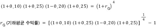
The interpretation: each year, you earned that $r_G$ rate. That’s the lens here.

This is also called the time-weighted average return!!

Do you see why it’s time-weighted?!

Q1’s return affects Q2’s return.

Q1 and Q2 affect Q3.

Q1, Q2, and Q3 affect Q4.

Everything affects everything else like that — so yeah, time-weighted feels like the right name!!!!

(Honestly, every now and then the econ-eye gives me a fresh way of looking at physics, lol. So refreshing.)

Dollar-Weighted Return

This one factors in the scale of assets under management while it’s averaging.

Why does that matter? Stick with me 60 seconds and it’ll click.

Easier to start with the definition, because once you see the formula it kinda hits you all at once.

So: the dollar-weighted average return is the internal rate of return (IRR) of a project. The textbook says it’s “the return rate that makes the present value of the cash flows realized by the portfolio equal to the initial cost of setting the portfolio up.”

…what does that even mean.

OK let’s make it concrete. Say the initial investment is $1M.

Period 0 (now): cash flow = -1.0

Period 1: -0.1

Period 2: -0.5

Period 3: +0.8

Period 4: +1.0

And IRR as a formula:

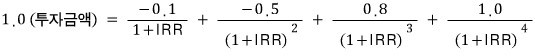
You just solve that equation for IRR. Done.

Now — what does it actually mean?

Here’s how I’d put it:

“What return rate do you need, exactly, to break even?”

Right?! Because every term is a ‘present value’ conversion at its respective period. So —

“At this return rate, you break even.”

That’s the level of meaning I’d assign to it.

Which is to say — it kinda functions as a benchmark return rate. A reference point.

---

OK so we’ve got all these different ways to compute average returns. Now — for things like mutual funds, which method is the standard? In other words, how do you annualize a return?

That’s what we’re looking at next. And honestly, after going through all those average flavors, this part should land easier.

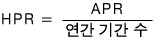
There are two layers of annualization, and you do them in sequence.

First, using a simple-interest approach, you build a rate that represents “how much return was earned over some period overall.” Then to answer “OK so if we converted that to one year, what is it?” you compute the annual percentage rate (APR).

Then on top of that, you build a factor that says “alright, at that APR, in some specific sub-period, how much return is that equivalent to?”

That second one is the effective annual rate (EAR).

Formula makes sense, yeah?

And saying “we hit that APR” really means — for each sub-period (this is where you account for stuff like bonds paying interest twice a year), how much return did we effectively earn? When you bake compounding in:

FYI — bonds pay interest twice a year, so $n=2$. Mortgage-backed securities pay monthly, so $n=12$.

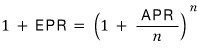
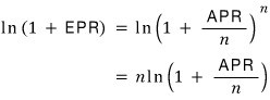
Now, let’s take the log of both sides. We don’t wanna deal with that exponent sitting up there.

We’ve made it this far. Time for a bit of math.

I’m not gonna derive this directly — the derivation itself isn’t really the point right now.

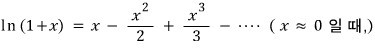
Following the Maclaurin series principle (which is just the Taylor series centered at $x=0$), we get this:

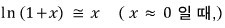
Which is to say,

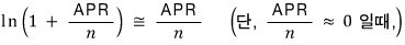
And rearranging the earlier equation using this:

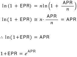
Boom — this relation links APR and EPR!!!~~~

Let’s run one example and call it a day.

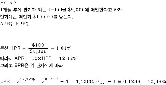
Since we used a Taylor approximation, our answer is off from the textbook’s exact calculation by about 0.02%. Close enough.

---

Originally written in Korean on my Naver blog (2016-04). Translated to English for gdpark.blog.