Statistical Theory, Risk, and Risk Premium

Last time we talked about returns. Cool. But there’s this nagging question that won’t go away.

“Hmmmm…”

Like — couldn’t you deviate from the average return?

What’s the probability of deviating? And by how much?

If we’re going to ask questions like that, we need to be able to answer with stuff like “it’s x%” — you know, an actual number.

Which means… we need to talk stats for a bit.

Don’t worry, I’m not about to launch into a stats lecture. It’s not like I grinded statistics super hard and know it deeply — I’ve used it a handful of times, that’s it. And honestly? The stats we need here is so embarrassingly basic that any high school stats textbook covers it. So… T_T T_T T_T

ANYWAY!!!!

To answer “what’s the chance a return of such-and-such happens?”, apparently step one is to build scenarios.

Scenarios are simple. Instead of treating things as some crazy continuous variable and slicing it into a million tiny pieces, you just go:

“severe recession,” “mild recession,” “small bit of growth,” “full-on boom” —

four broad-strokes situations like that, and you eyeball a rough probability for each.

Then for each one you write down something like “HPR will probably be around this much~”

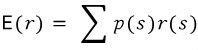
Once you’ve got that, you can compute the expected return. And expected value is exactly what it sounds like — the value you expect.

What’s the difference between this and the average????? → The flavor’s a little different but mathematically they’re the same thing.

(In my experience, when people are talking about stuff that already happened they say “mean,” and when they’re predicting stuff that hasn’t happened yet they say “expected value.” Same math. Different vibes.)

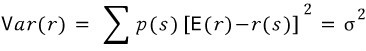
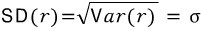
Once you’ve got the expected value, from there you can also compute variance and standard deviation.

Variance = the average of the squared deviations (squared distances from the mean). Standard deviation = the square root of variance.

Variance, as “average of squared distances,” tells you how wiiiide the Gaussian is spread out. Standard deviation? Since variance squared everything (which weights big distances extra hard), taking the square root cancels that out, so std dev means roughly “the average distance from the mean.”

(Spoiler — there’s also the average of the cube of the deviations, the average of the fourth power, and in fact the average of the n-th power. In stats these are called the “k-th moment about the mean.” We’ll get to what the 3rd and 4th moments mean in a sec, lets gooo.)

Anyway, this is intro stats stuff, so let me just dump the definitions and keep it moving.

OK so that’s how it goes. But notice — this whole logic chain has been built on the assumption that the probability function is a Gaussian, right?

One of the perks of the Gaussian is — normalization? standardization?

Yeah. The fact that you can standardize it.

And what’s so great about that?

You can compute things easily using deviations. Stuff that would otherwise be a mess of ugly numbers becomes super clean once you push it through standardization.

I mean… if you don’t standardize, it’s not like all analysis grinds to a halt.

(In physics it doesn’t seem like people standardize all that much. Also — the situations where Gaussian actually applies aren’t that many anyway… unless you’re dealing with something built out of Bernoulli trials, i.e. normalizing a discrete distribution, maybe…)

Anyway, from high school probability and statistics class, you’ll remember:

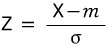
You do this variable substitution to normalize.

When you do this substitution and rewrite the Gaussian, the mean becomes 0 and the standard deviation becomes 1… which doesn’t just happen by accident — you deliberately chose the substitution to make it come out that way.

A Gaussian with mean 0 and standard deviation 1 is called the standard normal distribution.

If you do this, you can carve out a kind of guideline within, say, a 95% probability scenario — a “boundary line” that captures 95% of outcomes. In investment-speak, this boundary is called value at risk, or VaR. (Apparently the R is capitalized to distinguish it from Var, which is variance.)

But as I said up top — this whole thing is built on the assumption that returns are Gaussian. So you also need to check whether the Gaussian assumption actually holds in real-world investing.

And what’s the yardstick for measuring how far a distribution drifts from Gaussian?

It’s exactly those “3rd and 4th moments” I teased earlier.

The 3rd moment — the average of the cubed deviations — measures skewness.

The 4th moment — the average of the fourth-power deviations — measures kurtosis.

The Gaussian is bell-shaped and symmetric, right? Mirror image around the mean. So you can use how much it fails to be symmetric as a measure of how far it is from Gaussian — that’s skewness. (Skewness of the Gaussian = 0.)

And kurtosis?

Hmm. Roughly, “pointiness.” Numerically, it’s “how often extreme values show up compared to a normal distribution.” Bottom line — for a Gaussian, kurtosis = 0. And here’s a graph of something with kurtosis ≠ 0:

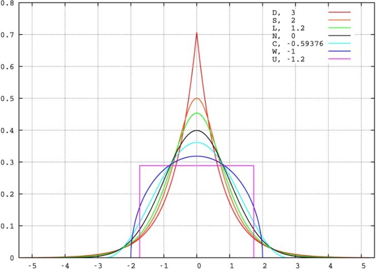
Pretty intuitive, right?

OK and skewness — same deal, Gaussian skewness = 0. Graphs of skewness ≠ 0:

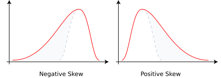
Negative skew is leaning toward the positive side, and positive skew is leaning toward the negative side!

(Note. The variance of a Gaussian tells you how wide and flat the bell is. Don’t mix it up with kurtosis.)

So where do we actually use this stats machinery?

When you read the textbook once, you might be like “wait, isn’t this thinking way too simplistically?” Maybe. But still, let me sum up what the book is going for.

Out there in the world, there’s something called the risk-free rate.

A return you’re guaranteed, no matter what.

Roughly: the deposit rate you’d get sticking your money in a bank, or the return on a T-bill.

Returns like those carry zero risk, and you can lock in at least that much.

So why would anyone invest in anything else? Because the risk-free rate just isn’t sexy enough. People dive into riskier assets, taking on a little risk, hoping for more return.

When you do that, there’s some amount you earn over and above the risk-free rate, right?

That extra chunk is called the excess return!!!!!!

It’s a real term — file it away~~

(Imagine you walk into a bank. They tell you if you invest in some product, expected return is 6%. Just leaving it in a deposit, the interest is 2%. The excess return for jumping into that other asset = 4%~ heh.)

But here’s the catch — no matter how juicy the expected return, nobody actually wants to take on insanely high risk, right…?

So another question. The products that securities firms sell — are their risks always priced fairly???

Nope.

Some products carry not-much risk, with not-much return to match. Others carry serious risk, with seriously high return as the trade-off. And you can’t seduce people into the high-risk stuff with high return alone.

So there’s something the seller offers — or the buyer demands.

The risk premium.

“If you’ll take on this risk, we’ll throw in a little extra^^”

“I’m taking on this risk, so toss a premium on top, please.”

That’s the vibe.

And to figure out how much risk premium is fair — that’s where the stats from above comes in.

For some portfolio,

the expected return is

$$E(r)$$

and let’s say the volatility of that asset is

$$\sigma$$

Wait — why is standard deviation suddenly getting called volatility????!!!~~~

OK so. Standard deviation is basically the (de-weighted) average distance each outcome sits from the mean. Which means you can also read it as

“this is roughly how much the value can swing”

— and that’s why it gets reinterpreted as volatility.

Note. To be more precise, standard deviation in a Gaussian is the width of the distribution out to where the probability has fallen to

$$e^{-1/2}$$

times its peak.

OK, now say the risk-free rate is

$$r_f$$

Then the excess return is

$$E(r) - r_f$$

(For a risk-free portfolio,

$$\sigma = 0$$

obviously.)

So the size of the risk premium that should be paid is exactly

$$E(r) - r_f$$

— that’s what this number is trying to say.

Now, if you want to ask: with what probability does this excess return actually show up? With what probability do you lose it, or earn it? — what’s the right yardstick?

Right. It’s

$$\sigma$$

— the volatility.

You can evaluate how much risk you took on for that excess return, with volatility as the ruler.

So when people talk shop, it makes sense to use volatility as the basis for “how much risk burden did I take on” — i.e., when demanding a risk premium, using std dev as the yardstick: “I’m bearing this much risk!!! How much premium are you adding!!!!”

The risk premium you get in exchange for accepting one unit of standard deviation — that’s called the Sharpe ratio.

$$S = \frac{E(r) - r_f}{\sigma}$$

Why “Sharpe”? Because a guy named William F. Sharpe came up with this measure in 1954. Dude apparently got the Nobel in Economics in 1990. Not bad.

Anyway, just to say it one more time — S is:

“For an excess return of

$$E(r) - r_f$$

how much risk did you eat???”

— it’s the risk premium per unit of risk taken on. That’s the interpretation.

OK so, wrapping up.

Take volatility into account → evaluate how much “risk” you’re carrying right now → use S as the ruler → evaluate the “risk premium.” That’s it!!!

---

Originally written in Korean on my Naver blog (2016-04). Translated to English for gdpark.blog.