Inventories (4): Lower of Cost or Market (LCM) [CFA Level 1 Notes #7]

Feels like we’ve been grinding on inventory forever,

but honestly it only dragged out because of FIFO and LIFO,

and really, at this point we’ve covered initial recognition (when you first buy inventory, how do you set the cost → tack on all the incidental costs until it’s ready for its intended use) and

derecognition (when inventory leaves, how does it leave → as COGS).

Let me plug the last gap.

You buy inventory, and then 12/31 rolls around and you have to put together financial statements,

and at that point, do you just leave the inventory sitting there at whatever you paid for it? That can’t be right, right?

So the question is how we do “subsequent recognition.”

Like I said, we need to think carefully about the inventory that didn’t get sold and is still sitting around,

i.e., the stuff that’s recorded as Inventory on the B/S.

Let’s say it’s Samsung Electronics’ mobile division.

They’re cranking out the Galaxy 10 (what Galaxy are we even on these days? I’m an Apple person so I honestly have no idea….),

and all the cost up to the point where it’s Ready for Sale gets recorded in won as the inventory value of the Galaxy 10,

let’s say one Galaxy 10 cost 500,000 won to make.

But now the foldable Galaxy has dropped, right?

If the Galaxy 10 units that still haven’t sold are about to be dumped at 300,000 won,

in that case, should the Galaxy 10 sitting on the B/S stay at its 500,000 won cost?

Or should it be flipped over to the 300,000 won market price??

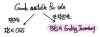
The answer! “Whichever is lower — that’s what it becomes."

Inventories recorded on the B/S follow a subsequent recognition where you swap them to the lower of historical cost and market value,

and this is called the Lower of Cost or Market approach — the LCM method (lower of cost or market method).

And knocking the value down per LCM is called a write-down.

Hold up!!!! Market Value — what we’ve been calling “market price” — actually has a few different flavors.

Realizable Value, the “how much would I pocket if I sold this right now?” approach: the Net Realizable Value (NRV) is realizable value minus stuff like commissions and selling costs.

(NRV is going to get mixed up with Fair Value later, so to be a bit more precise — NRV assumes the company is selling ’through its normal operating activities.’ It’s not just “throw it on the market and see what happens.” So NRV is an entity-specific measurement,

and the number you get can be totally different depending on whether Megastudy is selling the asset or the little math tutoring place around the corner is selling it.)

Replacement Cost, the “how much would it cost to buy this again right now?” approach.
Value in Use, the “shouldn’t we look at the present value of the cash flows this asset will throw off in the future?” approach.

And a few more.

So we said for inventories we use Lower of Cost or Market,

but which concept of market price exactly?!

It’s different under IFRS vs. US-GAAP.

(Since CFA is an American exam, you have to know both IFRS international standards and US-GAAP. T_T)

Under IFRS, MV (market value) is defined as NRV.

So in this case we don’t even call it Lower of Cost or Market,

we call it Lower of Cost or NRV.

IFRS goes with NRV because, for inventory, the whole point of acquiring it is Sale.

That is, End Inventory cost = min(original acquisition cost (Historical Cost), NRV).

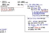
Now under US-GAAP, the default is also NRV for MV,

but in the LIFO case…………… it gets a little messy!!!!!!!!

MV is taken as Replacement Cost,

with the ceiling (upper bound) on MV being NRV, and the floor (lower bound) being NRV − Normal Profit.

(Here Normal Profit just means normal profit — easiest way to think about it is the profit that covers the BEP.)

Ugh…. this is a mess, but let’s at least take a look at why they set it up like this.

First — the values that inventory sitting on the B/S is allowed to take shouldn’t be able to blow past some level or crash below some level (otherwise it’s Abnormal), so they had to set upper and lower bounds. When you compare against Replacement Cost (RC — what you’d pay to buy it right now),

the intuition is “if the price you can sell it for right now is higher than the price you’d pay to buy it right now, that’s weird,”

so the rule becomes “you can’t go above the sell-it-now price as your ceiling, right?”

(If the sell-price right now were higher than the buy-price right now, literally everyone would just buy everything right now and flip it… total nonsense situation.)

The floor on RC is saying “the RC, where you buy it right now and sell it right now, should still leave you with normal profit — an RC that would let you earn more than normal profit is a weird value, no way you can get it that cheap,” and that’s the logic for the lower bound.

In other words — the “Abnormal” range they carved out is really just a common-sense range.

The way US-GAAP handles this is what they call Lower of Cost or Market!

But we’re people prepping for an exam,

and if you try to reason through that range every time during a timed problem,

you’re not winning the time attack.

For calculating LCM under US-GAAP when LIFO is being used, it’s a bit faster to just know the shortcut.

Take Mid(RC, NRV, NRV − Normal Profit), the median of those three, as MV.

Then, since it’s Lower of Cost or Market, compare that MV against Historical Cost (HC) and take the smaller of the two as the inventory cost on the B/S.

So as one formula:

(under US-GAAP) LIFO inventory cost = min( Mid(RC, NRV, NRV − Normal Profit), HC )

Messy, right? Honestly, since it’s CFA material, this is already the simplified version.

If I tell you the real truth — which, for your mental health, “you might want to skip” — (under IFRS):

To prep the End B/S, first check whether the inventory quantity on the books (book quantity) matches the actual quantity.
There’ll be a discrepancy. When you do a physical count and come up a little short, that also has to be expensed, and that kind of expense is recorded as “inventory shrinkage loss.”
Quantity done, now the price — compare original acquisition cost vs. NRV and see whether a write-down is needed.
Multiply the actual quantity (after all that) by min(acquisition cost, NRV) and record that as End Inventories…

Anyway!!!! The point is — this is how we pin down the cost that gets multiplied by quantity for inventory on the Ending B/S!

That’s what we just wrapped up.

OK, now let’s look at how a Write-down plays out in the financial statements.

If we decide the inventory amount on the debit side of the B/S is too high and yank it down,

the credit side has to come down by the same amount too — but where does that reduction land?

Yep yep, it comes out of Retained Earnings.

Because if a valuation loss pops up from applying LCM, that loss gets recorded as cost of sales in the current period.

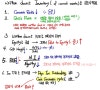
So what does a Write-down do to ROE?????

ROE is Return on Equity, calculated as Net Income / Equity,

and LCM drops both net income and equity.

Lowering both the numerator and denominator gives you the results above.

(You can prove this arithmetically, but there’s no need to — and no need to memorize it.

If you’re in the exam hall, just scribble 2/3 and then subtract 1 from both numerator and denominator, check whether 1/2 is bigger or smaller than before, and use that.)

Stuff like this —

a situation where numerator and denominator move in the same direction —

is the classic example of “you can’t just eyeball it.”

Let’s blast through one more quick example and move on!!!!

Current Ratio = 1.3

Quick Ratio = 0.7

Working Capital = 30,000 — say we’ve got a company like this.

If Cash received in advance comes in, how does each ratio shift?!?!

At first glance you might go “oh?!?! Cash is up?!?! Everything gets better?!?!??” — nope, that’s a miscalculation.

Because of this,

A Current Ratio that’s greater than 1, when numerator and denominator both go up by the same amount, gets smaller,

and a Quick Ratio that’s less than 1, when numerator and denominator both go up by the same amount, gets bigger.

And Working Capital stays put, which matches common sense.

OK so, this time,

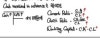
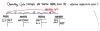
there’s more to say about Write-downs.

NRV of inventory dropped hard, it got revalued lower,

so we applied a Write-down, and both inventory and Retained Earnings came down.

But then more time passes, and the NRV of that inventory bounces back up.

In that case, should we write up the amount we’d previously written down??????????

The verdict:

US-GAAP does not allow it.

IFRS allows it, but the cap on how far up you can go is Historical Cost — that’s the rule.

(In practice, I hear this almost never actually happens. Once it goes bad, it just goes, apparently.)

As a diagram it looks like this.

Done~~~

<Not-important aside>

Whether under IFRS or US-GAAP, there are cases where writing up above historical cost is allowed —

commodity-like products (agricultural & forestry products, mineral ores, precious metals) —

for stuff like that, because the swings are huge and the impact on corporate value is significant, accounting treatment that recognizes the ups and downs is apparently applied.

(This is what’s called ‘biological assets’ territory, and for biological assets specifically they’re measured at NRV from initial recognition onward, and continue being measured at NRV after that. So even if you paid 10,000 won for it, if you go to initially recognize it and find the NRV is 8,000 won, a loss can pop out right at the moment of initial recognition. :-)

This is judged unimportant for CFA exam purposes, but since the material mentioned it briefly, I’m dropping it in here lightly and moving on.)

Alright, we’ve seen that inventory recorded on the B/S can go up or down.

And we’ve seen how ROE shifts when LCM gets applied.

Let’s dig a little more into how other financial ratios are affected,

so we’re harder to fool when we stare at financial ratios going forward.

The headline ratio is the Inventory Turnover Ratio (Inv T/R),

and if Inv T/R is high, we’d usually say the company is using its inventory efficiently.

But just because Inv T/R is high, you can’t unconditionally say “ah, efficient.”

Because if inventory got Written Down,

a write-down simultaneously jacks up cost of sales AND knocks down inventory,

so the inventory turnover ratio itself explodes upward…. shudder.

So if you’re looking at a company whose Inv T/R has gone up, you’d better check whether the reason was inventory write-downs from LCM, you see, heh.

- For reference -

With that vibe in mind, let’s take a look at how other financial ratios get hit.

Days Inventory Outstanding and Cash Conversion Cycle in number 6 just showed up out of nowhere….

We’ll get into these in more detail later, OK?!?!!??

It’s stuff you’ll get just from hearing it once roughly here anyway,

but I’ll come back to it later, haha haha.

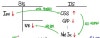
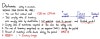
There’s this thing called the Operating Cycle.

The reason companies buy inventory is to sell it.

The reason they sell it is to make money, haha haha.

Operating Cycle = the period between a company buying inventory and actually collecting cash.

Let’s say the company transacts on credit.

First, the company buys inventory on credit.
Then it pays off that credit amount.
Then it sells the inventory, also on credit,
and some time later collects on that credit, right???

The time from 1. to 4. is exactly what’s called the Operating Cycle.

Drawn out as a diagram, it looks like this.

From here, along with the Days Inventory Outstanding and Cash Conversion Cycle I mentioned above, a few concepts come out.

Days Sales Outstanding: period ③, the time from sale occurring to cash being collected.

Days Inventory Outstanding: periods ①+②, the time from inventory purchase to sale.

Days Payable Outstanding: period ①, the period from inventory purchase to paying off the credit.

Cash Conversion Cycle: periods ②+③, the stretch where the company effectively has no cash.

The rough way to compute these periods is actually just to use the turnover ratio,

which is why the relationships in number 6 fall out like they do,

and based on my study notes, when I hit this topic again on p.48 I’ll bring it up one more time!

Change in Accounting Principle.

A company’s been using LIFO for its cost flow assumption, and then goes “you know what, let’s align our disclosures with international accounting standards! Let’s start writing our financial statements using FIFO!!!”

You can’t really block that from happening, right????

So when a company says it’s changing its accounting policy,

should it rip up all the existing financial statements and retroactively apply the new policy (retrospective method)?

Or should it apply it going forward (prospective method), starting with the financial statements published from now on????

Just thinking about it, the retrospective method feels more rigorous, more “correct.”

But then, if you think about it some more —

say we’re looking at Company A’s Q2 financial statements, and the inventory numbers look pretty good.

Except you can’t trust them anymore…..

because the suspicion creeps in: “wait, couldn’t these numbers get changed later through retrospective application??”

So the accounting standards drew a line — certain things get retrospective, certain things get prospective — and

the intuition you want to have is:

“if something that almost never changes does change” → retrospective method.

“if something that can change all the time changes” → prospective method.

And here, Accounting Principle belongs to the “almost never changes” bucket, so it’s subject to retrospective application.

One type of change under that Principle is the cost flow assumption (FIFO, Avg, LIFO).

So if you flip that cost flow assumption, the company has to rip up and resubmit all its past financial statements too!

Later on, Change in Estimation falls into the “can change often” bucket,

and that one uses prospective application.

The classic case shows up in depreciation —

say you bought a piece of machinery for 100 million won, and when you bought it you set the useful life at 10 years and residual value at 1 million won, and you’ve been running depreciation every year while using it,

and then it’s determined that a super-ultra-saiyan upgrade would massively boost sales, so the company spends 50 million won on the upgrade.

With that, the company can extend or shorten the useful life, and can also change the residual value.

This falls into Change in Estimation, and for that, prospective application is used.

The main content’s all done,

and for the remaining odds and ends, I’ll just sub in photos of my handwritten notes!

(Yes, I admit it, pure laziness…. ^^)

Whew, inventory is finally donnnnnne haha haha haha haha haha haha haha haha.

Next up — tangible assets!!!!!!!!!!!

Originally written in Korean on my Naver blog (2021-05). Translated to English for gdpark.blog.