Level 1 Content Review

Alright, shall we kick off Level 2? I trust you’ve completely formatted Level 1 out of your brain and come back fresh, right? lol Let’s rebuild the average concepts from scratch and march in properly!

OK first, let me throw in a thumbnail.

Arithmetic Mean

Brainlessly add everything up, divide by the count — that’s the average we use most in everyday life. The arithmetic mean! So what does this arithmetic mean actually mean~?

Say I made money day by day like this: 10,000 won + 20,000 won + 10,000 won + 30,000 won + 50,000 won + 10,000 won + 20,000 won. Now ask: “Over the course of 1 week, how much can I say I earned per day on average?”

The thinking goes: “How much would I have had to earn per day ($x$) so that the total comes out the same as 10,000 + 20,000 + 10,000 + 30,000 + 50,000 + 10,000 + 20,000 above?” Set up the equation:

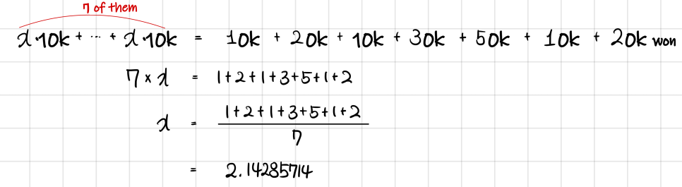
Aha — so over the week I earned roughly 21,428 won per day~

But what if the subject were returns?

If over 1 week my stock returns were 1%, 2%, 1%, 3%, 5%, 1%, 2%, can I just say I earned about 2.14% per day on average? Absolutely not, right? lol Because we’re talking returns in % units — your account doesn’t grow by + addition, it grows by × multiplication. So we have to express the per-day earnings as the average of multiplication!

So what’s the average of multiplication…?

Geometric Mean

Let me explain the geometric mean with a rectangle story. I had a farm: 9 wide / 3 tall. To expand, I bought up the surrounding land. Now it’s 18 wide / 9 tall — meaning, I expanded 2× horizontally / 3× vertically.

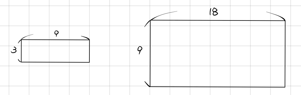
Aha! So I expanded by the average of 2 and 3 → 2.5× this time!! — nope, you can’t say that. Both directions have to expand by the same factor of $x$ times, so:

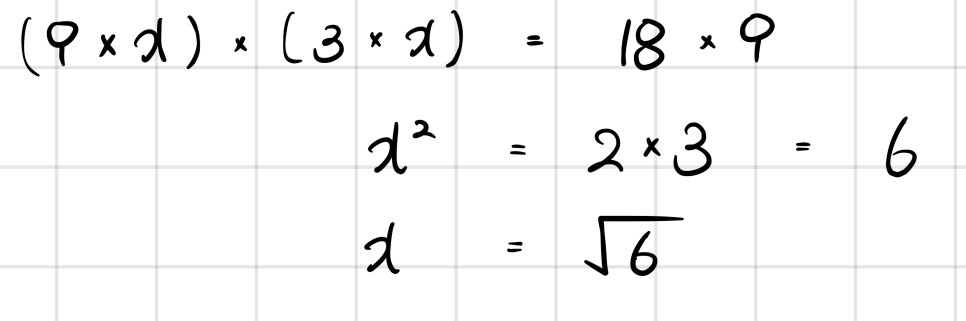
You have to say the width and height each expanded by an average of $\sqrt{6}$ times!

The reason we write returns as 10%, -10%, etc. is precisely to say it’s growing by multiplication. So if a 100,000-won account earns 10% on day 1 and -10% on day 2:

• Day 1: 100,000 → 100,000(1+0.1) = 110,000
• Day 2: 110,000 → 110,000(1-0.1) = 100,000(1+0.1)(1-0.1) = 99,000

It ended at 99,000. So when we ask “what % return/loss did I see per day on average?”:

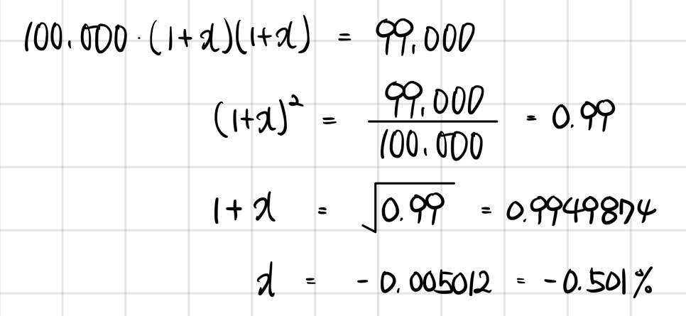
You have to say it amounts to an average daily loss of 0.501%!

(10% & -10% counts as a loss, lol. The world of stock investing is a scary place — what’s the point of earning 10% if the next day you’re down 10% and it’s all wrecked~)

So why did I drag us through all this multiplication talk?!

To revisit the Yield Curve content from Level 1.

Term Structure

What we usually just call “interest rates” — the Spot Rate and Forward Rate. And YTM (Yield-to-Maturity) refers to the “annualized average return” that a price is expressing, given that price. And of course, the average here is a geometric mean.

(YTM is more of a return concept than an interest rate concept. But because it’s a return from promised cash flows rather than the expected cash flows you deal with in stocks, we call it a Yield.)

OK, let’s build this up little by little starting from spot, just like in Level 1.

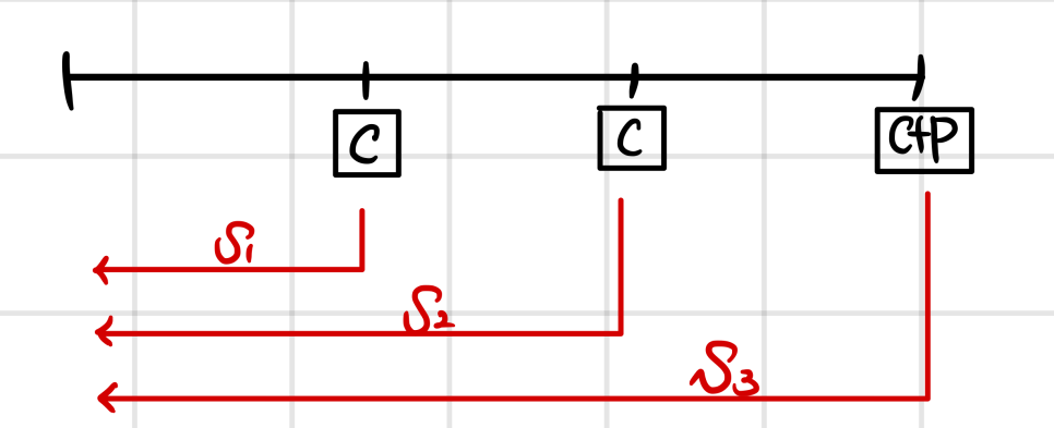
Going one at a time: buy a 1-year zero-coupon bond → annualized average return is $s_1$. Buy a 2-year zero → annualized average return is $s_2$. Buy a 3-year zero → annualized average return is $s_3$.

$s_1$ is your money growing over 1 interval at an “average speed” of $s_1$. $s_2$ is your money growing over 2 intervals at an average speed of $s_2$… Because of this, the spot rates $s_1, s_2, s_3$ are all “annualized average” concepts.

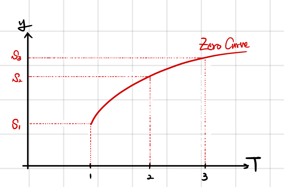
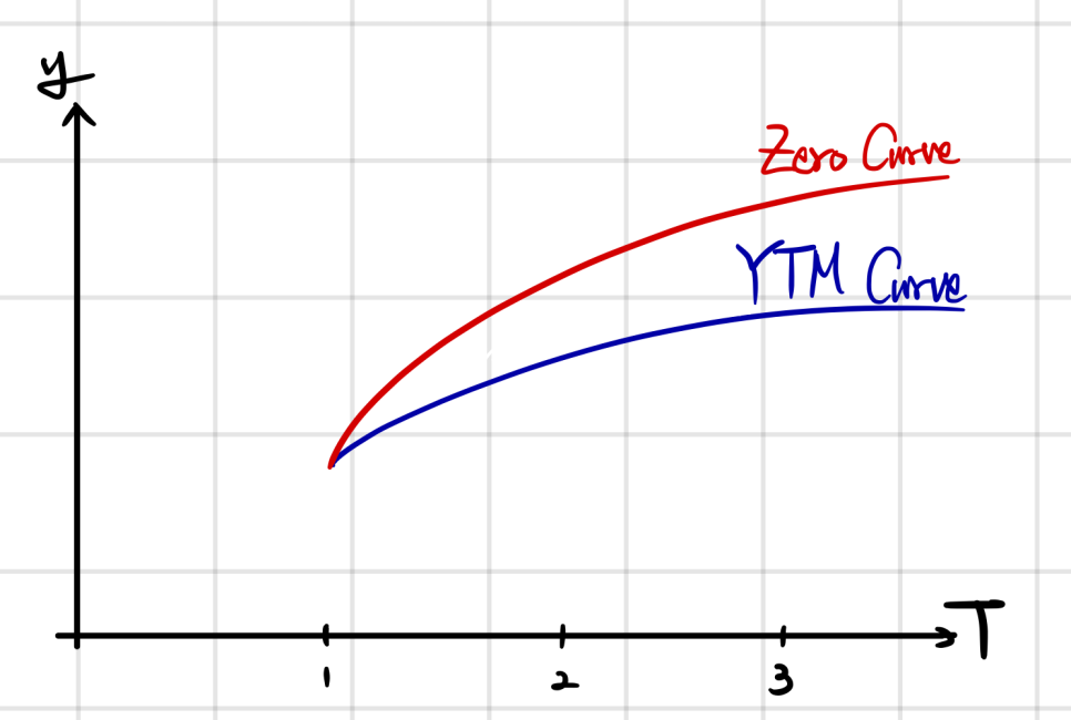
In the market, $s_1, s_2, s_3, \ldots$ can all be observed, and plotting them on a $T$–$y$ axis gives us what we called the Spot Curve, or Zero Curve.

The price calculated from this is the no-arbitrage theoretical price:

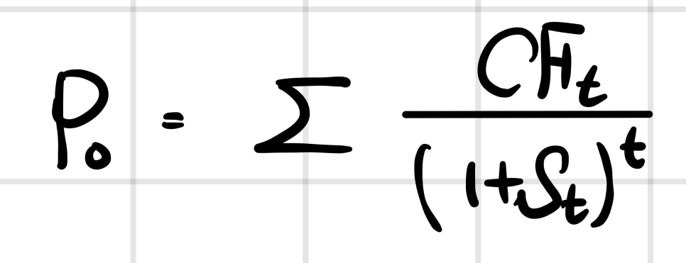
We studied that this is called the “No Arbitrage Price (or Theoretical Price).”

Now, say I bought a bond at that price. Actually, saying “a bond price is given” is the same as saying “the YTM is given,” because all the future cash flows are fixed — so the return you’d earn collecting them all the way to maturity can just be calculated. So price given ⇔ YTM given. (And the other way around: YTM given ⇔ price given.)

So how do you actually compute YTM?

YTM is calculated through this kind of process. And what does it ultimately mean…

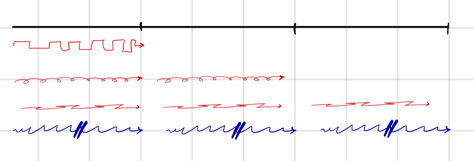
It ends up being: you assume the speed at which money grows is the same (= YTM) across every interval, and you compute the “average” return across the whole investment horizon.

Here, if $s_1 < s_2 < s_3$ (upward sloping)? Then $\text{YTM}_3 < s_3$, right?

So if the spot curve is upward, YTM gets drawn below the spot. Conversely, if spot were downward, YTM would sit above spot.

Forward Rate

The Forward Rate refers to the interest rate for a period of length $y$ starting $x$ periods from now.

Let’s go with this notation. Anyway — the reference point is not now, it’s a future point in time!

The theoretical forward rate is calculated so that no arbitrage opportunity arises from the present. Drawing it out:

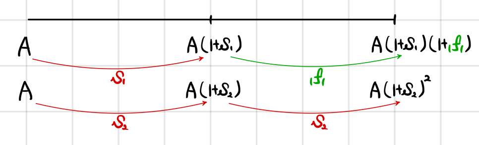
For no-arbitrage, the upper line and lower line have to be equal:

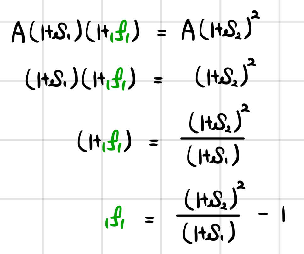
And there’s the forward rate.

Now, the same question — is it above or below spot?

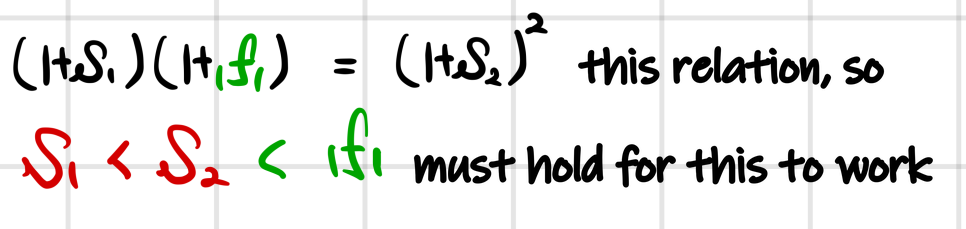
So, if spot is upward sloping, the Forward Curve is drawn above the Spot Curve. If spot is downward, it’s drawn below.

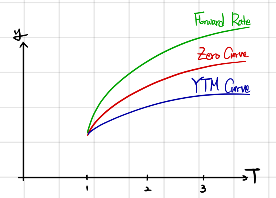
The forward rate computed this way is said to be implied in the spot — hence the name Implied Forward Rate. So if you’re given only spot rates, computing the forward rate for an $n$-year period starting $m$ years from now is trivial.

(Just shows you how much information is packed into the spot rates…)

That’s also why people say it’s worth eyeballing the term structure when you want to know how the economy is expected to play out going forward.

* CFA tip! This will save your life on problems — in the CFA world:

• Economy expected to be bad → downward sloping or Inverted
• Economy currently bad → upward sloping

Solve every problem with this and you’re set.

But, like… when you actually look at current real-world interest rates?

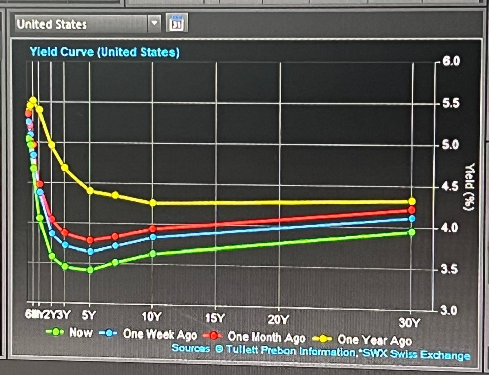
What on earth am I even studying ;_; lol

One more thing — Spot Rate and YTM are “annualized average” concepts (and YTM ends up being the average of the underlying spot rates). But Forward Rate is not an average from today — it’s a per-unit-period concept: the rate for one future slice of time (still quoted per year, like any rate). Make a note of that.

In other words: spot is the standard, but because spot is being viewed through the annualized-average lens… if you want to slice things up period by period, you have to look at Forward.

Expected Return & Realized Return

Quick thing to internalize: actually earning the YTM over the whole holding period requires that “reinvestment happens at YTM." (The YTM itself is just the rate that matches the price; it’s the realized return that needs the reinvestment.)

Say I buy a bond with Par = $1,000 and coupon rate = 10%, issued at par. Issued at par means coupon rate = YTM, so YTM = 10%. Meaning my money grows at an annualized average of 10% for 2 years. So the $1,000 I put in at $t=0$ should become $1{,}000(1+0.1)(1+0.1) = \text{\textdollar}1{,}210$ after 2 years.

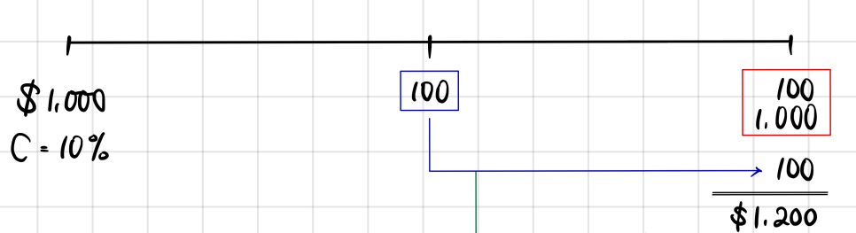
But it falls a little short?! How on earth does this work?

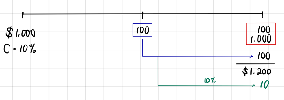
There has to be an assumption that the 100 you receive as a coupon in the middle also gets reinvested at the YTM of 10%.

Let’s double-check by pulling it back to the other side.

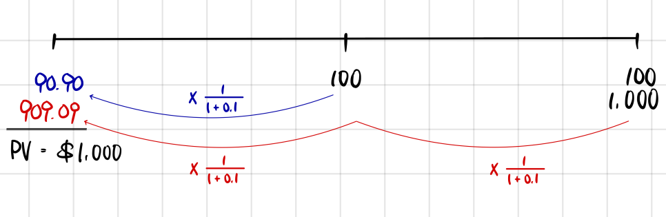
In that PV (present value) calculated this way, actually…

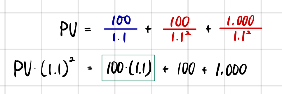
reinvestment income is sitting right here… What this means is — that calculation

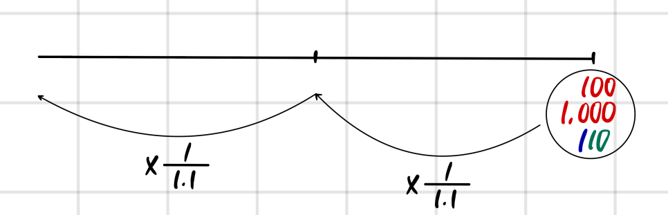
treats this situation as equivalent.

And in reality, over the actual investment horizon, you might want to plow the mid-period coupons into something that yields around YTM, but no such investment might exist. Or maybe you find an even better one…

So — the expected return estimated by YTM and the actually realized return can absolutely differ.

Just keep that in the back of your head…

Ah, writing this is hard? lol When am I ever going to finish this post? lol Welp, off to go study AI… bye~~

---

Heads-up. The figures here are the original notes, slips and all. A few things to watch for:

• In the timeline picture, $100/1.1$ rounds to 90.91 (the picture cuts it to 90.90); with 90.91 the two present values add up to exactly 1,000.