The Arbitrage-Free Valuation Framework

Yaaaaa finally Chapter 2~~~~~~

Now we start picking up the new Level 2 stuff!!!

This is gonna be fun!! haha

Anyway, let’s gooooo~~

Chapter 2. The Arbitrage-Free Valuation Framework

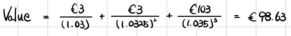
When we compute the theoretical price of a bond, what we’re really doing is valuing it at a price where no arbitrage shows up — the law of one price.

But here, unlike Level 1, we leave the door open: rates could go up, rates could go down… and we value bonds by modeling rates with a Binomial Model. heh heh heh heh

Hmm.. so in derivatives, through put-call parity,

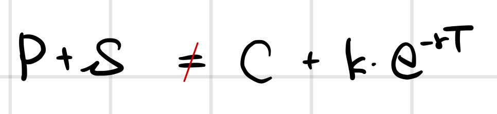
we already saw how, the moment that equality breaks, an arbitrage opportunity pops up.

But in the bond market — what kind of setup gives you an arbitrage opportunity?

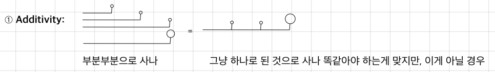
There are two types: ➀ Value Additivity (the value of the whole differs from the sum of the values of the parts) ➁ Dominance (one asset trades at a lower price than another asset with identical characteristics)

➁ Dominance:

When somebody says “characteristics” about a financial product without specifying, it’s basically shorthand for the return–risk characteristics.

So — same return-risk profile but different price? → That’s when an arbitrage opportunity is sitting there.

(Put-call parity, by the way, was a Dominance-type arbitrage!)

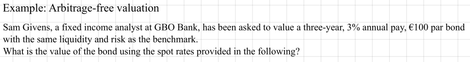
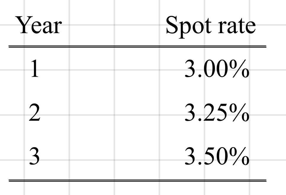
Since the characteristics line up with the benchmark, we can just reuse the same numbers we used to discount the benchmark and value it that way.

Binomial Interest Rate Tree Framework

If we just take the spot rates the market hands us and use them straight up — well, once you’re given the $s_i$’s, the ${}_{i}f_{j}$’s are all observed too,

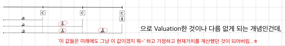
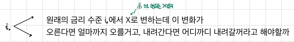
But in reality ${}_{1}f_{1}$ and $s_1'$ are going to be different, and honestly we can even predict ahead of time that they’ll be different, so when we compute present values now, we want to leave enough room for the possibility that things shift.

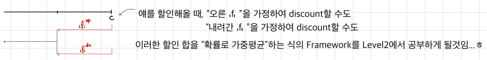
That said — ${}_{1}f_{1} > s_1$ still holds, right? (assuming upward sloping)

So be careful: don’t model the tree in a shape like

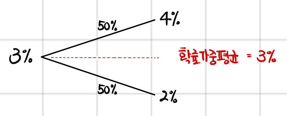
If everyone’s expectation is that ${}_{1}f_{1}$ = 4%, then at the bare minimum the model has to give you a probability-weighted sum that equals 4%.

In other words, drawing the tree properly:

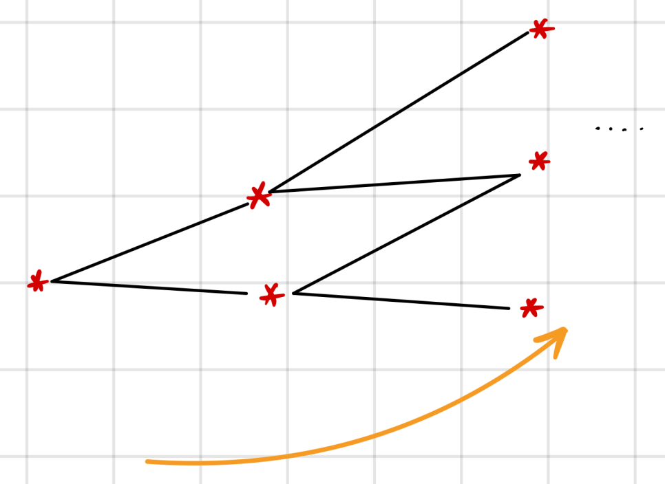
The tree itself ends up being an upward-sloping model — that’s what this means!

One more thing. If you have $s_1$ = 3%, ${}_{1}f_{1}$ = 4%, the number of trees that probability-weight back to 4% is not just one — meaning the “angle,” the spread of the branches, is also a key parameter of the model. And the number that captures it is volatility! (Next chapter we look at embedded options, and that’s where this becomes super important!)

So — option-free bonds we can value with just a plain spot rate curve. But for bonds with embedded options, future rate changes are going to affect the probability of the option getting exercised, which in turn affects the future cash flows.

Bonds without embedded options? Spot curve, done. (So when you’re working problems, also know not to go through unnecessary suffering on option-free bonds! haha)

But callable / putable bonds? The movement of interest rates is hugely tied to whether the option gets exercised, so these absolutely have to be valued through a model that has up-scenarios and down-scenarios baked in!

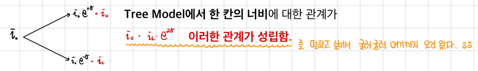
Anyway — the model we’re going to be working with from here on is the Binomial Interest Rate Tree, and it assumes that next period the interest rate has an equal probability of landing on one of two possible values. (50:50 probability!!! Notice — when we priced options on stocks, we computed and used a risk-neutral probability separately. That part is different here!!!)

OK, let’s actually get into the binomial model, one of the interest rate models. Most basic question first: if we had to define “what is an interest rate?” in one phrase, what would we say? Think about it ⇒ couldn’t we just call it “the time value of money”??? ok ok, interest rate model — let’s go!

So, button one: there are two things we need to lock down first about the Binomial Interest Rate Tree Model.

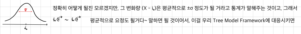
Baseline assumption in finance: the distribution of returns is Lognormal. What’s that, simply put?

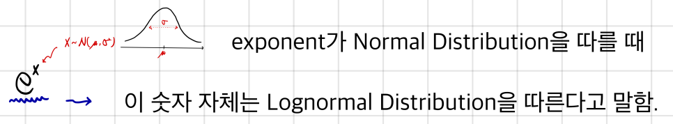
And in finance the convention is — it’s returns, not stock prices, that get assumed normal. And here, interest rates can be thought of as returns, and apparently it’s better to assume these follow a Lognormal distribution too!

(I tacked on an appendix at the very back from “probability theory I studied,” covering the lognormal section.)

And the use of this model also reflects the following:

But… honestly, at this stage it’s hard to explain how it gets reflected nicely.. that’s content that’s going to click naturally later!!!

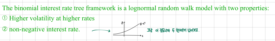
What we want to walk away with right here is that the framework we’re going to be using has two features: ➀ Higher volatility at higher rates ➁ Non-negative interest rate

Let’s just remember there are these two!

Originally written in Korean on my Naver blog (2024-11). Translated to English for gdpark.blog.