Binomial Trees, Part 2

Last time we had the tree handed to us — already built — and we just played with it. This time? We’re building one from scratch. That’s the whole gig today.

And we’re gonna do it while keeping in mind how wide the branches spread out in the tree ($2\sigma$).

1. The interest rate tree has to spit out arbitrage-free values for the benchmark security.

Remember how we ended up with a present value of $102.999 last time? Cool. But what if that’s not the price actually trading in the market?? Then the tree’s wrong. It has to be redesigned so the value it pops out matches the market price.

This whole “tweak the parameters until the answer matches reality” routine has a name — it’s called the Calibration Process.

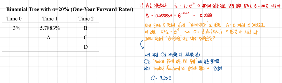
2. Like I said before, adjacent forward rates in the same period are two standard deviations apart, calculated as $e^{2\sigma}$.

Yeah… literally already covered this. Moving on.

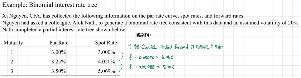
3. The middle forward rate in a period is approximately equal to the implied one-period forward rate for that period.

OK so circling back to the earlier example — remember we had 1f1 floating around as 7.1826% and 5.3210%? The average of those two doesn’t have to be exactly equal to anything, but it should be approximately equal to the implied forward rate you’d calculate from the spot rate.

Approximately: my read is, when you’re actually solving a problem, just use $e^{2\sigma}$ and call it a day lol

Anyway — once we’ve got the interest rate tree built like this, we’re golden. Either we run Backward Induction like before, or — when that doesn’t fly — we go Pathwise valuation. Either way, we get our present value~

Originally written in Korean on my Naver blog (2024-12). Translated to English for gdpark.blog.