Valuing Option-Free Bonds with the Binomial Model

Ah man, it’s been forever since I opened my blog.

I’ve been… insanely busy. Like, life-eating busy.

(I’m still busy right now, actually — but I kicked off a code run and I’m just sitting here waiting on the results, so I figured hey, might as well crack open the blog. hehh)

Lots of stuff happened in the meantime. Good things, bad things,

I’ll tell you about all that later. heh heh heh

Anyway — back to Level 2!!

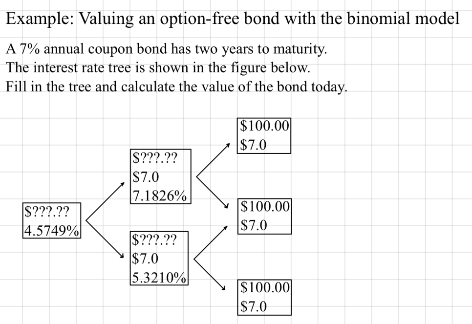
Valuing an Option-Free Bond with the Binomial Model

OK so we’re jumping straight into valuation using the model.

But first let’s get a rough feel for this thing called Backward Induction, then we’ll walk through an example.

Backward induction is the process of valuing a bond using a binomial interest rate tree.

What that’s actually saying is —

assume you’re holding the bond all the way to maturity no matter what. Start from the very end, where you collect your final coupon and principal —

then pull forward one step at a time, valuing the present value as you go —

that’s backward induction.

You’ll get it once we run an example!

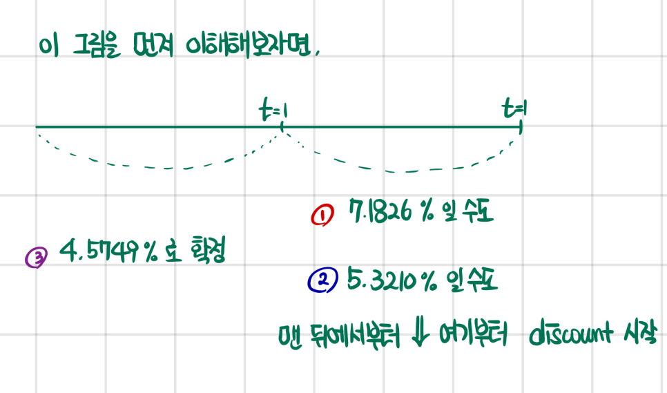
So at each node, you’ve got a spread of possible interest rate outcomes,

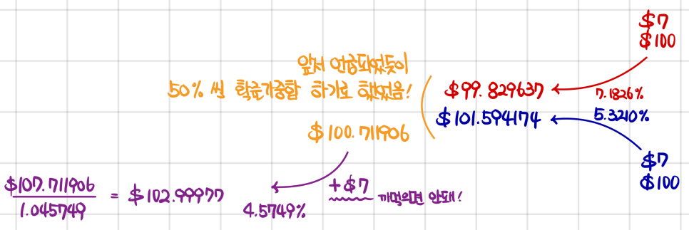
you pull each one back, take the probability-weighted sum, and that’s the value of the bond at that point in time.

And since you also collect a coupon at that node along with the bond,

you carry the coupon along too — don’t forget it — using backward induction that keeps dragging everything forward —

just keep discounting all the way back to the present~~~

That right there — that’s Backward Induction!

Now — it’s not like you have to do it this way!!!

There’s also something called Pathwise Valuation.

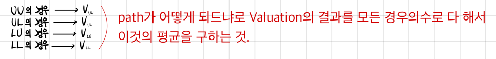
Even doing it this way, the answer comes out exactly the same — so why is it that these always end up matching???

It’s because we’re taking a 50% probability-weighted sum, that’s why the same value pops out. (An arithmetic mean already assumes equal probability, after all.)

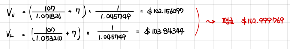
If you run this example the Pathwise way, the only possible outcomes are two — U / L — so… (Because the very first edge is basically already locked in.)

But hold on — if the answer’s the same, why on earth do we have to learn yet another methodology…?

Path Dependency

It’s because when the cash flow is path-dependent, backward induction doesn’t work..

In those cases, you’ve gotta go pathwise!!

Picture a mortgage pool that got formed back when rates were 6%, then rates dropped to 4%, climbed back to 6%, and dropped again to 4%. A bunch of homeowners are gonna refinance the first time rates dip.

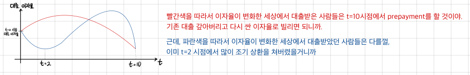
So in a situation like that, here’s how it gets explained:

Because of path dependency of cash flows of mortgage-backed securities, the binomial tree backward induction process cannot be used to value such securities. We instead use the Monte Carlo simulation method to value mortgage-backed securities.

The book uses MBS as its go-to example for path dependency,

so I used the term MBS too — but obviously path-dependent cases aren’t limited to MBS.

Anyway, in those cases you’ve gotta use Monte Carlo. But… Monte Carlo is really just Pathwise valuation in the end, isn’t it…~

Originally written in Korean on my Naver blog (2024-12). Translated to English for gdpark.blog.