Term Structure Models: CIR, Vasicek, Ho-Lee, and KWK

OK so now we’re getting into actual models.

Up until now, we only learned the basic ground rules for building a Tree. Now, on top of those rules, we want to study the stochastic process side — how interest rates actually move, how they get generated. The various methodologies that model rate fluctuations by defining a stochastic process.

Only the famous ones, heh.

Broadly, two camps:

➀ Equilibrium Term Structure Models

➁ Arbitrage-Free Models

And since past exams have loved asking “what are the characteristics of each model” — let’s lock those characteristics in.

Equilibrium Term Structure Models

attempt to describe changes in the term structure through the use of fundamental economic variables that drive interest rates

The two famous ones here are the CIR (Cox-Ingersoll-Ross) model and the Vasicek model.

Both are single-factor models — they use only one factor.

And that one factor? Both pick the short-term interest rate.

CIR model

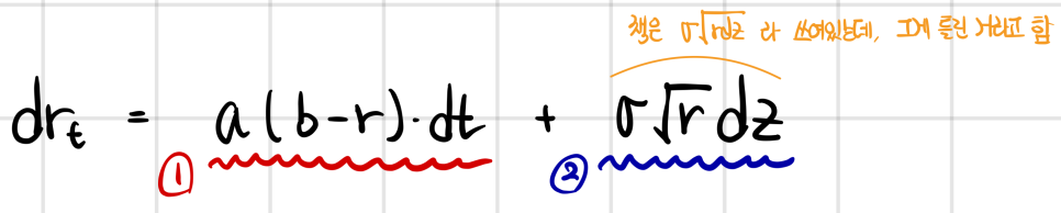
• a: speed of mean reversion parameter (the mean-reversion constant)
• b: long-run value of the short rate (the long-run average rate)
• r: the short rate (current rate)
• dz: a tiny random-walk kick (dz ~ N(0, dt))

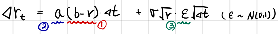
This is the continuous-variable version. If you walk through the math and convert it to the discrete version

(same vibe as converting the stock-price model to discrete when you were doing Black-Scholes;;)

Let’s get this intuitively.

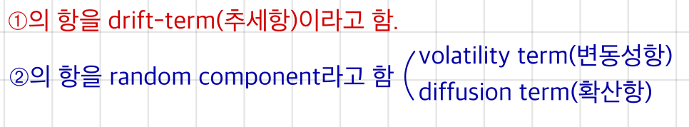
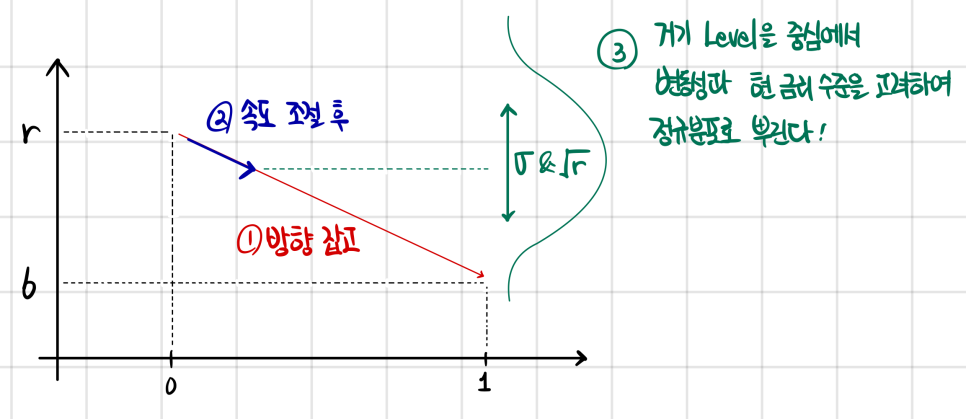
➀ pushes the direction of the next interest rate move toward the long-run average — but it doesn’t just yeet it straight there in one shot. Instead, ➁ sets how fast it walks toward that long-run average.

So that gives you the target level for next period’s rate. And then, centered on that target, you spread things out according to a Normal distribution.

The width of that spread? That’s σ (volatility). (Along with the current rate level r doing some work too.)

That’s the CIR philosophy for modeling the next period’s rate change. And it’s a model that’s actually used in the real world — not just academic flavoring with no practical bite.

It also shows up on the exam a lot lol (most important lol… worldly studies, gotta eat…)

Vasicek Model

Pretty much the same shape as CIR.

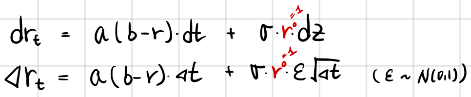
The Vasicek Model is the one where the random kick doesn’t reference the current rate level.

I wrote the exponent as 0 (so it collapses to 1) just to make the side-by-side with CIR easy to eyeball.

The actual difference: in CIR, if the previous period’s rate gets estimated as a negative number, the random term in the next rate estimate goes imaginary — and your model breaks because rates suddenly become complex numbers. Vasicek doesn’t do that.

So CIR can blow up, Vasicek doesn’t. Sounds like Vasicek wins, right?

But — Vasicek pays for that by allowing negative interest rates outright, which becomes its own weakness.

Anyway. The Equilibrium Term Structure Model approach is basically: is the rate above or below its long-run average? — and steer it toward where it ought to be. That’s why they slapped the word “Equilibrium” on it, apparently!!

The exam asks whether you understand the meaning, so going at it conceptually is the right move. And honestly, even if you asked me to — why is this mathematically valid, how is it proved, how is it logically derived — nah… that kind of thing, go enroll in a financial engineering program. If I had to do that here, I never would’ve started CFA in the first place lol.

Arbitrage-Free Model

If the Equilibrium Term Structure Model carried a “To-be” philosophy,

the Arbitrage-Free Model is more of an “As-is” philosophy.

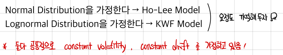
This camp also has two: the Ho-Lee Model and something called KWF (Kalotay-Williams-Fabozzi), but…

we can’t really go deep on this part lol.

For CFA, it feels like the exam can only really ask about characteristics anyway lol.

Ho-Lee Model

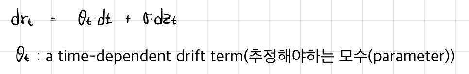
Derived using the relative pricing concepts of the Black-Scholes model,

this model assumes that changes in yield curve are consistent with a no-arbitrage condition

Black-Scholes itself was a formula built on a no-arbitrage condition — and this is basically saying the same thing, but applied to interest rate changes: assume a world where arbitrage in rate movements isn’t possible.

KWF Model

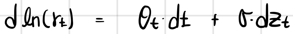
This is literally just “Ho-Lee, but do you Log it or not.” That’s the whole difference.

So in the end, $dr_t$ — the change in the rate —

Originally written in Korean on my Naver blog (2024-12). Translated to English for gdpark.blog.