Economic Feasibility Evaluation of Investment Projects [Corporate Finance I Studied #7]

We learned about cash flows earlier,

and once cash flows are measured like that,

we have to do economic evaluation of the investment proposal… because we need to judge which cash flow is better and which is worse, right?

So the idea is, we measure the cash flows of vaaaaaarious projects,

and then evaluate those cash flows

This kind of work is called ’economic evaluation’, and once you do economic evaluation,

you get a clear picture of which investment proposal to pick,

and which one to reject

So there are said to be 6 methods for doing economic evaluation on cash flows

Average rate of return, payback period method, net present value method, profitability index method, internal rate of return method, and capital allocation — 6 methods like that

Average rate of return method (average rate of return : ARR)

You take the expected annual average profit from the investment

and divide by the annual average investment amount to compute the figure

This is a value computed entirely from accounting profit, so it’s also called the “accounting rate of return”.

However, for that calculation

let’s point out there’s a little tip to this calculation.

Ex. 8.1

Equipment with a purchase price of 35 million won has a useful life of 5 years,

and no salvage value.

If you invest in this equipment, the annual net profits by year are estimated to be

Net profit

200

500

800

600

700

Since there’s no salvage value and depreciation is constant,

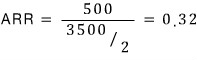
The annual average investment is

At the start of year 1, 3500 is invested, depreciation of 700 is taken off, so year-end investment is 2800 → average of the two = 3150

Start of year 2, average of 2800 and year-end 2100 → = 2450

Start of year 3, average of 2100 and year-end 1400 → = 1750

Start of year 4, average of 1400 and year-end 700 → = 1050

Start of year 5, average of 700 and year-end 0 → = 350

The average of the five is (3150+2450+1750+1050+350)/5 = 1750, which is exactly half of 3500, yep!

ARR is easy to calculate and convenient, but

the fact that it doesn’t use cash flow and uses accounting profit instead

means — and here’s the poison — that it does not consider the time value of money….

This is said to be a truly fatal weakness.

Payback period method

The ‘payback period’ among these words refers to “the period during which the expense spent as the investment amount is recovered from the initial investment point”

In other words, the shorter the payback period, the better! — that’s how it’s evaluated

The reason it can be evaluated this way is because a shorter payback period is seen as boosting the firm’s liquidity

Especially when the future is soooo uncertain, there’s a benefit to securing liquidity first, so this method can be used!

Ex. 8.2

Year

Cash flow

-5000

1000

2000

1000

3000

In a case like this, the ‘payback period’ is, after the initial 5000 investment goes out,

how much longer until it all comes back in — that’s what you look at,

first, after 3 years 4000 has come in, and the situation is that only the remaining 1000 needs to come in,

and thinking that the remaining 1000 comes in after just 1/3 of year 4 passes

payback period = 3 + (1/3) years = 10/3 years

that’s how it gets evaluated

Well, you set up a payback period that the company itself decides as the standard,

and if it’s shorter than that, Pass, if longer, Fail! Just give it an F lolololololol

But this payback period method, while it has the advantage of being as easy as the ARR before,

the first problem is that it doesn’t consider the period ‘after the payback period’

So, if you considered beyond the payback period, you could get results different from the payback period method…. that’s the problem

And like ARR, this one also doesn’t consider time value… T_T

bye 2

Net present value method

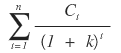
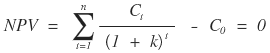
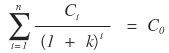
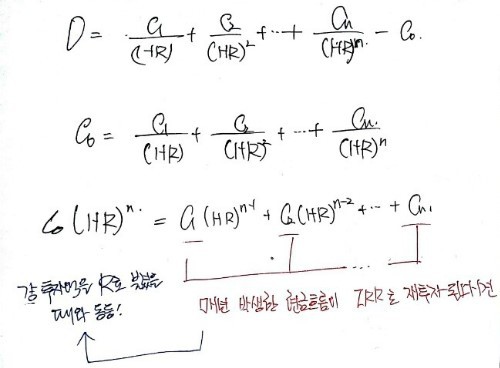
Net present value (net present value : NPV) is the sum of the present values calculated by discounting all cash flows arising from the investment at an appropriate discount rate, minus the initial investment cost

That’s called NPV!

In a formula, you can write it like this.

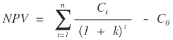
Here, k is the ‘minimum required rate of return’, which means ‘cost of capital’

Cost of capital, as the ‘minimum rate of return’ that must be realized through investment, is scheduled to be covered later in Chapter 13.

Chapter 13 is going to be a ‘game of finding the right k’, but we’re still in chapter 8, so just get the gist and move on~

Here, let’s assume we don’t consider ‘risk’ and think of k as the risk-free interest rate~

If there’s no other risk, you don’t demand a risk premium — compensation for bearing risk — from the firm, so

the truly minimum required rate of return will just be the risk-free rate~

Ex. 8.3

Investment amount

-1000

500

300

400

200

(k=0.05)

Well, you bang out NPV like this,

and if a positive (+) net present value comes out, Pass

if a negative (-) net present value comes out, Fail! — that’s how to give it hehehehe

But, as you can probably catch from that formula,

assuming cash flows are known, it’s self-evident that the only thing affecting the NPV value is k

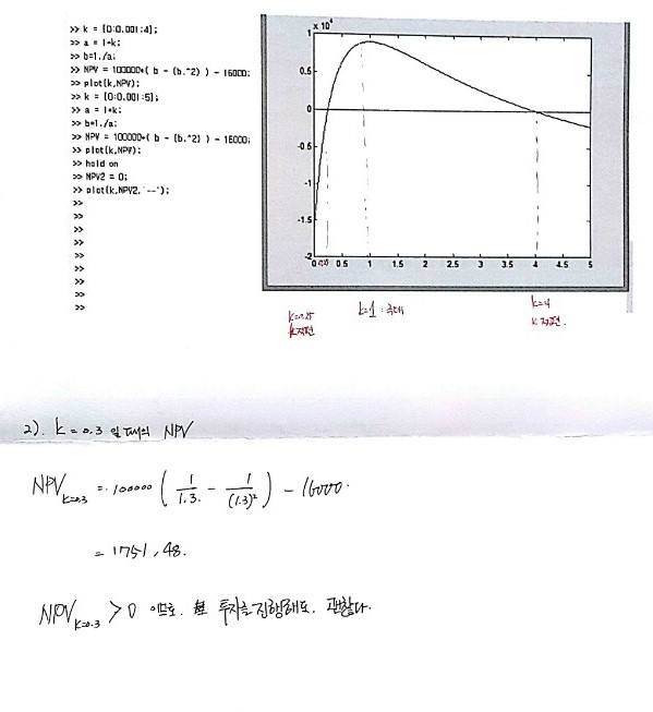
That is, we can extract the relationship between k and NPV!!!! (still assuming cash flows are known)

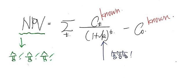
Since we know all those C_t, C_0 and such in this formula, even if you plug any arbitrary number into k

the corresponding NPV will come out — whoosh! whoosh! whoosh! — right?????

If you pair up those k and NPV values as ordered pairs

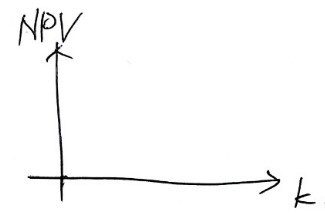
and plot them on this coordinate axis,

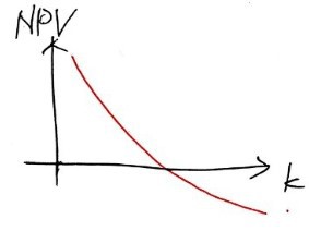
it’ll come out like this, right?????????????????

That is, what the curve tells us is that there exists a k that makes NPV = 0…

That k value we call IRR!

Internal rate of return!!!!!

Why it’s called this I’ll mention in a moment!

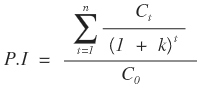
Profitability index method

Profitability index (profitality index : PI) is the value calculated by dividing the present value of future cash flows of the investment proposal by the initial investment cost

That is, as a formula it can be written like thiiiis

that’s what it means, and while doing the arithmetic is easy,

let’s dig into the meaning

of every 1 of the money I’m investing

per 1, what present value we get out — bam bam bam bam!!!

If the return per 1 is 0/57,

that means you invest 1 and get 0/57… meaning you can’t even pull out as much as you invested, which sends the signal that you shouldn’t invest,

and if the return per 1 is 1 or more, from then on it can be regarded as a signal that you can invest!

But,

the net present value method and the profitability index method can give rise to a contradiction

Let’s say we’re evaluating some investment proposals A and B

Net present value (NPV)

Profitability index (P.I)

400

700

320

1.8

300

600

300

2.0

Well, let’s suppose this is the case for investment proposals A and B

Then when evaluated by the net present value method, it leads to the judgment that A is superior,

and when evaluated by the profitability index method, it leads to the judgment that B is more superior…

Oh my god~

What is the fundamental cause of creating this kind of gap?

It’s because the scales of investment (C_0) between them are different.

So to properly evaluate A and B in this situation, you have to match up their investment scales

B’s investment scale is 1,000,000 won short, so to make it a situation where both invest 400,

you can close the gap by having proposal B simultaneously invest that 1,000,000 won in a risk-free asset while B is running, or deposit it in a bank, to match the investment scales.

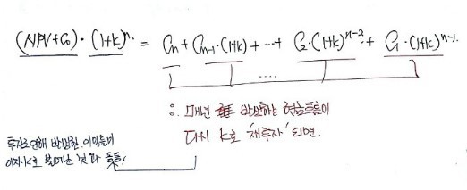
Internal rate of return method

Actually this is something mentioned earlier

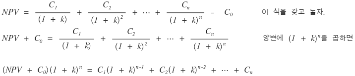
Internal rate of return (internal rate of retuen : IRR) — we said that the ‘discount rate k’ that makes NPV 0 is called the internal rate of return IRR,

that is

you derive the k value that satisfies this equation and call it the IRR value

(of course, C_t, C_0 are assumed to be known)

But, as was mentioned in other economics or finance fields,

solving this equation is considerably difficult…

Especially if n gets a little bigger, solving by hand is almost impossible…

But we learned the Bisection Method or the Newton-Raphson Method in financial engineering class,

methods for solving difficult equations like this, so we’re not worried,

ahhhhhhhh, so once you find the IRR of an investment proposal, how do you judge whether that proposal is Pass or Fail????

What does a high IRR mean →

“I can pull out profit without yielding even to a high cost of capital!!!”

Cost of capital, as said before, is the minimum rate of return that shareholders and creditors demand from the firm

A company’s IRR being high means it can endure even a high minimum rate of return,

and IRR being low means it can’t endure a high minimum rate of return,

so is the IRR of an investment proposal good when it comes out high? or good when it comes out low???

Higher is better!!!!!!!!!!

So, when comparing investment proposals, give Fail to the one with the lower IRR…!!!

Of these many kinds of investment proposal evaluation methods, the ones generally used most are

the net present value method and the internal rate of return method

Because both consider Time value

However, even when using these two together, they can also lead to opposite judgments, so

now we’ll look into why opposite results come out,

and what we should do then…

We’ll find that out and then leave this Chapter…

Anyway, like in the case of NPV and PI earlier,

by NPV, A is superior

by IRR, B is superior

the idea that this kind of result can come out..

So first, let’s look at under what circumstances such differing results get produced

i) When investment scale and cash flows differ.

When investment scale and cash flows differ from each other, naturally the evaluation results can differ.

Let’s say investment life is 1 year and the discount rate is 10%

500

800

1000

1500

Let’s take a peek at this situation~

If you do the calculation

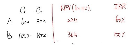
it comes out like this….

In this case, when evaluated by IRR, A’s IRR value is larger, leading to the judgment that A is superior,

but when evaluated by net present value, B’s BPV value is larger, leading to the judgment that B is more superior…

Why does this kind of selection discrepancy happen?……… can be

revealed surprisingly easily

Because if you draw the k - NPV net present value curve, you can see it at a glance

If you draw the NPV curve of A and the NPV curve of B on one coordinate axis

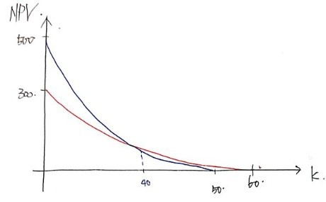
ah it’s a hand-drawn picture… please understand

Anyway, because the picture is drawn like this, you can see why the conclusion was that way

If it had been a situation where k=45%, the judgment through NPV value and IRR would be the same!!!

Anyway….. while the picture explains everything,

what we need to focus on is NPV….

Because IRR has no effect on ‘whether the investment proposal has a large present value or not’, no matter where it is!

We should just pick the ‘investment proposal with the larger present value’ at this current point in time

(ugh, so the essence is NPV, and the IRR method was just interfering from the side)

The fundamental cause bringing this kind of result……..

first, we can see that there’s a difference in the definitions of the two methods

hohohohoho

The essential meaning of NPV’s definition itself is actually

whereas IRR method

has in its definition the meaning

that it’s examined the minimum ‘interest rate’ under this assumption,

and the reason there’s a problem is that IRR differs for each investment proposal

so why is it being reinvested at R again?!??!?!?!

It could be that reinvestment at R might not happen again!!!

So following the net present value method

is what doesn’t confuse people!

Originally written in Korean on my Naver blog (2016-12). Translated to English for gdpark.blog.