Minimum Variance Portfolio

Picking up right from the previous post.

No intro.

​

​

Alright so anyway

Let’s take a look at how “risk” decreases by diversifying your investments across this and that​

Well, rather than risk decreasing, it might be better to say we can show ’the risk due to individual stocks disappears.'

​

​​

When there are 2 stocks in the portfolio​

The variance of the portfolio is

When n=3,

Up to here I don’t quite get the feel for it, but if we look at n=4,

What this is saying is,

let me write out the case for n = k

The number of terms where the risk from individual stocks affects the overall portfolio risk is k.

But the number of terms where the covariance affects the overall portfolio risk is

terms.

It’s going to be an overwhelming number….

So as the number of stocks increases, “the risk from individual stocks becomes meaningless.”

But the risk related to covariance remains.

I haven’t yet confirmed whether as the number of stocks increases, the overall portfolio risk gets smaller or larger, so I don’t know.

However, in terms of proportion,

I have at least confirmed that the covariance term takes up almost 100%.

Of course, since it’s the risk of the portfolio generated considering w_1, w_2, ~~~ , w_n too, it’s somewhat complicated.

But after leaving only the effect from the covariance@@@@@@@

if we adjust w_1, ~~~ , w_n to make that covariance-based risk as low as possible, we can make a veeeery fine portfolio~~

I think grasping it this way should work.

Then let’s take a very simple example and actually do the calculation.

Let’s say the number of stocks is 2, and the proportion both stocks take up in the portfolio is 50% each (w_1 = w_2 = 50% = 0.5)

and

let’s say this, and

like this

And we’re going to look at when the correlation coefficient between the two stock returns is 0, 1, and -1

A very interesting phenomenon is expected kekeke

First, when the correlation coefficient between the two stock returns is,

since it is

First, having seen it calculated this way,

I confirmed that it comes out smaller than the standard deviations of the two individual stock returns

But, that was just now with the correlation coefficient being 0, assuming the two stock returns are completely uncorrelated,

now we’ll look at the case where there’s a correlation.

Let’s say they’re in a very extreme correlation.

So I’ll do ρ = 1 and ρ = -1

Ah… even if you diversify,

depending on

this shows that it can be swayed.

What this means is…

//

“Yoo~~~ I did some investing this time, and I diversified!!~~”

//

“Oh really??? Show me hehehe how did you do it?!?!?!”

//

“Look at this~~~ Hyundai, Kia, Renault, and Ssangyong!!!~~~”

//

“Yeah, great diversification….;;;;;;;;;;;”

//

After seeing this story,

again

the 0.35 here being

the average of the standard deviations of the two individual stock returns coming out

kinda seems reasonable-reasonable, doesn’t it??? (since 50% each is invested)

Then let’s conclude like this.

In the case of,

when it is, it’s the largest, and

when it is, it’s the smallest!!!

It came out as 0.35 → 0.25 → 0.05.

From here on down,

I’m going to vary the ordered pair and look at the trend of how it changes.

Ah but, I didn’t calculate the expected return of the portfolio above,

this is

just weighted-summed like this, so I didn’t treat it as important.

But from here on down, I’ll calculate the expected return of the portfolio together.

Anyway, now

varying the ordered pair, let’s take a look at what the expected value of the portfolio return and the standard deviation are in each situation.

If I write out every single calculation step, it’d get insanely long, right?

Then I’ll throw out a table. Trust me! hehe

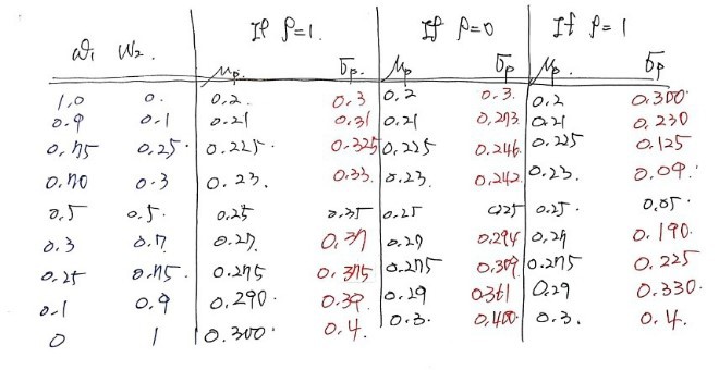
It comes out like this, they say.

Then pairing up the expected value of the return and the standard deviation of the return in each situation,

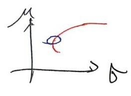
I’ll plot them as points pop pop pop on this coordinate axis!!

I’ll have the computer plot the points pop pop pop.

(blue: ρ=1, orange: ρ=0, gray: ρ=-1)

When I told it to plot the points

it plotted them like this

So I told it to connect them with lines here and there.

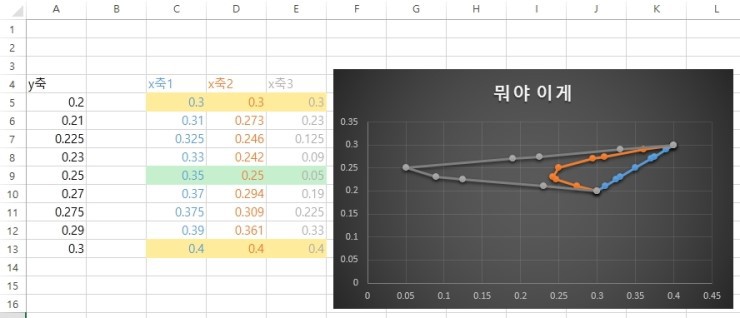
(blue: ρ=1, orange: ρ=0, gray: ρ=-1)

Ah…. the points aren’t being plotted the way I intended….lol

Right now

I divided the ordered pairs into 9 cases, but if I really subdivide them very finely

and consider many, many cases,

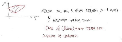
for the gray case, the points should be plotted like this

(blue: ρ=1, orange: ρ=0, gray: ρ=-1)

So I adjusted the data values a bit

and plotted one more point like this to manipulate it so the graph gets drawn the way I intended!!!

When rho is 1 and -1, they have the property of being drawn as straight lines!!!!!!

But, in that gray case where backward bending gets drawn, there’s a case where risk becomes 0????

Let’s just pocket this kind of fact.

So we can pull it out and use it when we need it^^

Anyway

Let me summarize.

I think it can be summarized like this.

When our portfolio is decided as a portfolio containing stock_1 and stock_2

Since the stocks are decided as stock_1 and stock_2, the correlation coefficient is decided as ρ_1,2,

if it had been stock_7 and stock_13, the correlation coefficient would have been decided as ρ_7,13 which is different from ρ_1,2,

but our choice was stock_1, stock_2,

so, meaning, right now

on this coordinate axis, one line has been decided, meaning

now we want to know the investment ratio w_1 for stock_1

and the investment ratio w_2 for stock_2.

That is, the moment the stocks are decided as i, j, “w_1 and w_2 that make it the minimum variance portfolio” will uniquely exist, right??

The ratio of w_1, w_2 at that minimum variance portfolio

will be represented by that blue point (point)

Where is the level of w_1, w_2 that gives us that point!!!!!

How do we find that!!!!!!!!!!!!!!!!!!!

Since the current situation is that we’ve decided to compose the portfolio with 2 stocks, stock_1 and stock_2,

it means ρ_1,2 has been decided, so

the portfolio variance is

this,

but currently, everything except w_1, w_2 is in a determined state!!!

Wow damn then there are two variables?????

That’s No No ~~~ we can merge it into 1 hehehe

since we have the condition w_1 + w_2 = 1

like this, now we have one variable

and the rest of the variables are now constants,

so we can find the w_1 that satisfies the minimum variance portfolio!!!

We just need to differentiate σ_p with respect to w_1, right?!?!!??!? since we just need to find where the derivative is 0

It only looks outrageously complicated

the arithmetic seems to be about 2nd-year-high-school level

Anyway, we found w_1 like this,

but do we have to find w_2 like this again????

That’s No NO ~~~~ it’s simple

P.S.

Did you know?

I’ve converted all my blog posts into pdfs

and am selling the pdf materials :-)

https://blog.naver.com/gdpresent/222243102313

Blog post pdf (ver.2.0) sale (Physics I studied, Finance I studied)

Purchase information is below ~​​​Hello! ​If there’s a part of the blog post you’re not satisfied with, or if it’s too over…

blog.naver.com

Originally written in Korean on my Naver blog (2016-12). Translated to English for gdpark.blog.