Efficient Frontier — Markowitz [Corporate Finance I Studied #11]

The content below covers material from my undergrad days.

You might think this is derived in a way that’s intuitive to understand,

but there’s a version that’s derived more mathematically rigorously.

https://blog.naver.com/gdpresent/223149758008

Efficient Frontier (efficient frontier, Markowitz) [QEPM as I studied it #intermission.] The efficient frontier you’ll run into with 1,000% probability if you study finance, the Markowitz curve, or whatever it’s called lol lol lol lol anyway https… blog.naver.com

After understanding it intuitively with the content below, if you want to handle it a bit more mathematically,

it might not be a bad idea to head over to that post :-)

(As a bit of a spoiler, if you understand it intuitively, you can’t even guess that the Efficient Frontier

has the form of the “hyperbola (x^2/a^2 - y^2/b^2=-1)” that we studied in high school.

But in fact, the efficient frontier is a hyperbola :-) )

Previously I looked at a portfolio made up of two stocks.

This time I’ll increase the count a bit

How much will I increase it by?? lol lol lol lol lol lol lol lol lol lol lol lol don’t be surprised

It’s “every stock in the world” lol lol lol lol lol lol lol lol lol lol lol lol

lol lol lol lol lol lol lol lol lol lol lol lol lol lol lol lol lol lol lol lol lol lol lol

This feels like elementary schoolers going “my dad is 100 years old!!!!!” lol lol lol lol lol lol lol

lol lol lol lol lol lol lol lol lol lol lol lol lol lol lol lol lol

Anyway, for convenience I’ll call it n lol lol lol lol

Alright alright alright alright alright alright alright alright alright alright alright alright alrightt

Here right in front of us we have stock_1 through stock_n………………

How many portfolio cases can we make using these as ingredients??????

→ Answer: a crazy ton

And to make matters worse, w_1 ~ w_n can be varied contiiiinuously

So there’s going to be an insane number T_T T_T

In any case

the portfolio’s expected return and return standard deviation are

calculated like this, right???

Then, for each individual stock

let’s think that values like these are all given,

and let’s think about considering all that crazy ton of cases here.

And of course the conditions are satisfied

So what I’m saying I’ll consider now — what exactly is it that I’ll consider?

The s that we plug into this equation computed like this

this case,

cases that are so numerous you simply can’t count them……!!!!!!

I’m saying that we’ll bundle the expected values and standard deviations that come out in each case into ordered pairs

, , ,~~~~~~

we’ll collect the countless data points that come out like this.

Gathering all the countless data

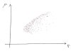
let’s plot them one by one by one, countlessly many points on this coordinate axis.

If we actually plot them

(Actually, I explained the logic here as above, but it seems like a lot of books explain it by continuously adding stocks to the portfolio one by one.

But I think it should be fine to explain it this way too, so I said it like above, but I’m slightly worried that there might be an issue here T_T T_T T_T if there is, please do point it out!)

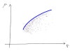
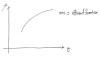
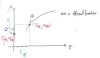
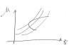
They say if we plot everything as points on this coordinate plane it looks like this,

(http://financetrain.com/constructing-an-efficient-frontier/)

Constructing an Efficient Frontier - Finance Train The concept of Efficient Frontier was first introduced by Harry Markowitz in his paper on Portfolio Selection (1952 Journal of Finance). The portfolio theo financetrain.com

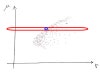
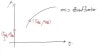
Now, let’s think about the ‘dominance principle’ for a moment.

At the same μ (return) level

that is, in this part here

among the portfolios belonging to the same return

Here, this

Is there anyone who would pick a portfolio on the right side, instead of the portfolio this blue dot points to??????????

The portfolio on the right side has the same return but higher risk

Probably, if humans were told to pick from that red range,

they’d pick the blue portfolio!

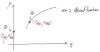
Of course the same holds at other return levels too.

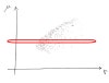
So I’m going to express it as: I collected only these blue lines and bundled into a set the portfolios that dominate all the other portfolios.

This line we call the

efficient frontier, and this efficient frontier means the most efficient portfolios among all portfolios we can make by mobilizing every stock in the world.

This Efficient Frontier was devised by American economist Harry Max Markowitz, who received the Nobel Prize in Economics in 1990,

so it’s also called Markowitz’s efficient frontier!!!

That’s as far as the Markowitz efficient frontier goes

so among those blue lines, which portfolio is the most efficient to pick?

The answer is (as I said in the previous posting) “it depends on the person”, isn’t it?

(please refer to http://gdpresent.blog.me/220890008630)

Portfolio variance, covariance matrix [Financial management as I studied it #9] In the previous chapter, if there’s some asset with μ and σ fixed, people, according to their individual utility function, … gdpresent.blog.me

Since the shape of each person’s utility indifference curve will be different

that is, since the degree to which they’re tolerant of risk will be different

the portfolio that maximizes utility on that curve will be different depending on the shape of each person’s indifference curve.

But here’s the thing. Actually, we can maximize utility even more.

That is, Markowitz was overlooking one thing.

If we think just a little more about the thing he overlooked, we can maximize utility even more.

What he overlooked — never mentioned once above — was the ‘risk-free asset’.

Above, risk-free assets weren’t considered,

but in the world, risk-free assets like ‘government bonds’ clearly exist

Considering this risk-free asset, we can increase utility a bit more

How do we increase it!!!!!!!

To understand this, we first need to take a quick look at how the expected return and return standard deviation of a portfolio that includes a risk-free asset are calculated.

Hmm…. I agonized a lot over how to phrase this to connect with the earlier content….

I’ll explain it like this.

You know those optimal portfolios we derived above?

Let’s call those portfolios “risky”.

It means a portfolio containing only risky assets.

Let’s say the expected return of this ‘risky’ portfolio is ,

and the standard deviation of its returns is .

And to this ‘risky’ portfolio, we’ll add a ‘risk-free’ portfolio made up only of risk-free assets

The expected return of this ‘risk-free’ portfolio is , and its risk is ,

but since its name is risk-free, its risk will be ~~

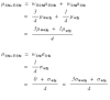
So the expected return of this newly composed “risky + risk-free” portfolio

will be determined like this~~~~~

But since this risk is….

it’ll be like this.

That is, the risk of a portfolio made up of a risk-free asset and a risky asset

is proportional to the investment ratio of the risky asset.

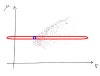
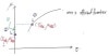
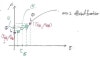
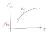
Let’s take the above story to the coordinate plane.

This is that efficient frontier from before, and here let’s pick one portfolio whose expected return is and whose return standard deviation is .

And we need to pick one risk-free portfolio too

Let’s say we picked them like this!!

And now, for the many cases of w_risky, w_risk-free investment ratios of the combined “risky + risk-free” portfolio

we’ll compute each corresponding

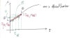
First, simply,

① All-in on the risk-free asset (w_risk-free = 1 = 100%), zero investment ratio on the risky asset

② Zero on the risk-free asset, all-in on the risky asset (w_risky = 1 = 100%)

in these cases, that point will be plotted here.

Obvious, righttt….?? lol? lol lol lol lol lol lol

Yup yup now then

w_1 = w_2 = 50% = 0.5

let’s say it’s invested 50% each like this.

Using the equation we derived above..,,,,,,,,, we can calculate it,

and a result that’s commonsensically obvious comes out.

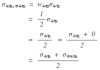
This is the explanation for point ③.

The ‘midpoint’ of μ_risky and μ_risk-free comes out as the result,

so I plotted point 3 like that above.

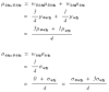
Point 4 works by the same principle.

It can be made as the midpoint of the standard deviations of the risky and risk-free assets.

So I marked point 4’s position like that

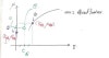
That is, when w_risky = w_risk-free = 0.5

the point that represents the identity of the ‘risky + risk-free’ portfolio is this point 5 here.

So then

when it’s ,

and

let’s only try when it’s…….

Let’s just do it;

when it’s

For the above two cases, I’ve colored the identity of the “risky + risk-free” portfolio

with green dots!!!!!

After dividing into 4 parts

weight of 3 on risky & weight of 1 on risk-free

After dividing into 4 parts

weight of 1 on risky & weight of 3 on risk-free

I think if you think about it this way, it should make sense that the points are plotted at the locations of those green dots.

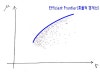
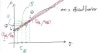
In conclusion, if we consider all w_risky & w_risk-free

and build a set of (σ, μ) for the “risky + risk-free” portfolio

unlike the shape of Markowitz’s efficient frontier

it becomes a straight line.

Then let’s go over one term.

The “straight line” that can be achieved by combining risky and risk-free assets, like just now,

is called the “Capital Market Line (CML)”.

Since this capital market line unconditionally passes through the point and the point

we can also derive it formally.

The line passing through two points

first, its slope is , and its y-intercept is

so following the equation exactlyyyyy

we can write it as !!!!!

Ah… but here’s the thing.

I drew the red line only up to that point above,

but actually the red line isn’t limited only up to there,

the extension line is also possible.

If you borrow more money at the risk-free rate (borrow more) and put your investment ratio in the risky asset above 100%,

then the extension of the line is also possible????

That’s why.

Now, by the way

up to the point of deriving this line

what;;;;; for;;;;;;; do you remember why I derived this line…?

Yeah…. to find a ‘portfolio set that maximizes utility more’ than the efficient frontier

is why I’ve been doing stuff like the above

and given that we’ve discussed this

this line is the “risky + risk-free” portfolio set that maximizes utility more

Why?!?!?!?!?!?!?!?! can a “risky + risk-free” portfolio that’s shaped like this

maximize utility more

Before, when we weren’t considering the risk-free asset,

the most efficient portfolio set we could choose was only this black line

and under this scope we kept maaaaximizing our utility function and

we could pick 1 portfolio that maximizes the utility function the most~

the logic was something like this.

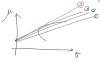
But, once we additionally consider the risk-free asset

we found out that the portfolio set we can form with the world’s (financial) investment assets is not only Markowitz’s efficient frontier,

but lines 1, 2, 3, and 4 can allllll be portfolios that exist in the world

so now there are even more cases where I can bring my utility function up against it.

But, while 1, 2, 3, 4 are all possible, there’s no need to try them all

and there’s no need to try with Markowitz’s efficient frontier either.

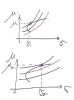
Because, line 4

‘dominates’ the efficient frontier, lines 1, 2, and 3.

So, before considering the risk-free asset

we’d have achieved the maximum utility U_1 using some portfolio that maximizes utility on Markowitz’s efficient frontier like this

once we consider the risk-free asset

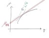
we can find a portfolio that maximizes utility with a larger U_2 than that, that’s the deal~

So now in the picture above, you can erase everything other than line 4, it doesn’t matter.

Erase everythinggg and leave only this line

and to distinguish this line from Markowitz’s efficient frontier

we call this line the “New Efficient Frontier”.

(They also call Markowitz’s efficient frontier the ‘previous efficient frontier’ in contrast with this~)

I feel like I explained super easy content at needlessly great length…

Anyway…. now the long-awaited CAPM

I’ll continue in the very next posting! hehe

Originally written in Korean on my Naver blog (2016-12). Translated to English for gdpark.blog.