Capital Asset Pricing Model (CAPM)

Now the content here is CAPM (Capital Asset Pricing Model)

But before getting into CAPM proper

when we were discussing Efficient Frontier in the immediately previous post

there were some things I didn’t mention, a few things I deliberately saved to talk about here.

I’ll mention those before going in.

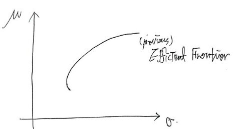
First, all the stocks that exist in the world are already determined.

This means the (Previous, Markowitz) Efficient Frontier is already, already determined.

Let’s say it’s determined like this.

But, after we derive the Efficient Frontier like this

we also thought about a risk-free asset, right????

But since this risk-free asset is also already determined as one that exists in the world

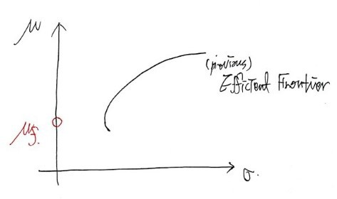
I’ll say the risk-free rate of the risk-free asset is determined like this.

The New Efficient Frontier created by this predetermined efficient frontier and risk-free interest rate

will also be determined.

Um.. so how the New was derived was

we said there’s a Frontier that maximizes each individual’s utility more than the Efficient Frontier does

and that Frontier, we could say, is a Frontier that maximizes human utility when the straight line drawn from that point is ’tangent’ to that curve

and the line drawn from this point that’s tangent to that curve is uniquely determined, right???? It’s already determined as 1.

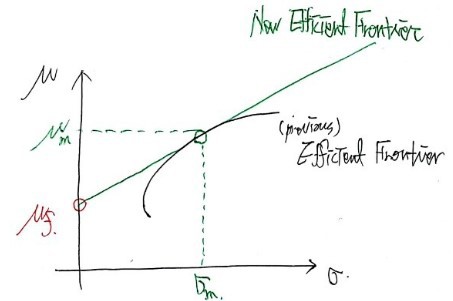
That is, some portfolio that belongs to the Efficient Frontier that builds the New Efficient Frontier

having this kind of expected return and standard deviation of return is uniquely determined.

We’ll call this portfolio the Market Portfolio!!!!

Then, this New Efficient Frontier can, in equation form,

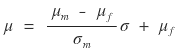
be expressed like this :)

Ah but, the mu and sigma without subscripts that are being decided now

are the expected return and standard deviation of return of the “risky + risk-free” portfolio, right????

So I’ll use the subscript p to write the meaning more firmly.

But here’s the thing.

Would it even be possible to construct such a portfolio?????

Finding such a thing would be hard,

Agh!!!!!!!!! But!!!!!!!!!!!!!

There’s something similar to that!!!

No no, there’s something that can be seen as similar in form

It’s the composite stock price index — things like the S&P 500, or in our country’s case, KOSPI 200!!

Why!! The composite stock price index can’t be said to move by reflecting the movements of all individual stocks in the world,

but still, because it’s an Index that bundles together the really big ones and represents the overall movement of that bundle

so thinking of the expected return and standard deviation of return of the composite stock price index

as these… that’s the majority opinion, and there are actually companies using this exact principle, so

it seems hard to think of it as too outlandish an assumption.

Then now we can head to CAPM (Capital Asset Pricing Model).

First, as it’s written in English, CAPM is the Capital Asset Pricing Model.

So this can be described as “a model that predicts the expected return commensurate with the risk of an asset (when the market is in equilibrium where supply and demand match)”

That is, it’s saying we’ll predict the expected return μ and standard deviation of return σ for an individual asset, and to say the meaning of ‘for an individual asset’ more directly, I’ll write mu and sigma with the subscript i as I explain.

But, what we’re going to predict it with is — as mentioned above — we’ll predict it based on the composite stock price index.

Uengh…T_T what’s this all of a sudden…T_T

First, there are assumptions embedded in the above model, and I’ll mention those first.

1. All investors participating in the market decide whether to invest or not using μ and σ as measures, and all investors are risk-averse investors.

2. The market is a perfect capital market. (No transaction costs like taxes, fees, etc.), and also individual investors are so numerous that each individual cannot affect the market price.

3. All investors have the same probability distribution for future asset returns (homogeneous expectation)

4. All investors can freely borrow and lend at the risk-free rate of return.

5. The investment period is a single period.

6. All publicly tradable financial assets are investment targets. (Excluding non-financial assets such as human resources)

7. The market is in equilibrium

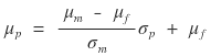
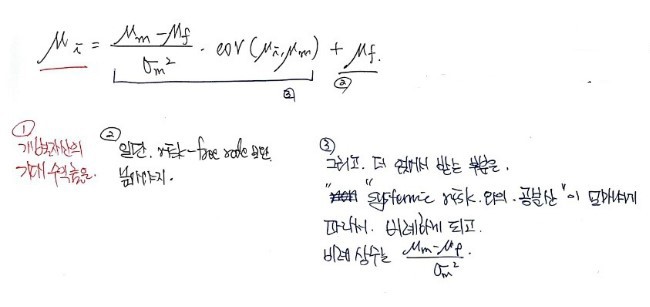
And I’ll rewrite the New Efficient Frontier equation from before.

The meaning of this equation can actually be viewed like this, right????????

You can view it in the order of 1, 2, 3 haha

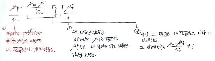
So my question is as follows.

Since the expected return and standard deviation of return of some portfolio composed of risky assets and risk-free assets are determined as follows

for the return and risk (standard deviation of return) of an individual asset

if we shing! plug in the risk of the individual asset as input, then μ_i pops shing~ out — couldn’t we just use it like this~~~

This is my question.

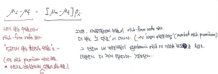
But here’s the thing. The equation for _p above

was New Efficient Frontier, whose target was the “efficient portfolio”.

An’nd the risk of the efficient portfolio is actually such that non-systemic risk totally flies away due to the diversification effect

and the remaining risk was only systemic risk (things like war, financial crisis — the overall… absolutely unremovable risk).

That is, since the risks of individual assets “can be eliminated”, attention shouldn’t be focused here

and the point is that attention should be focused on how individual asset risk is affected as the systemic risk changes.

So

it shouldn’t just go in pow! with only the name changed

and this guy should be adjusted by “how sensitively does it respond to the risk of the market portfolio that has only systemic risk (that is, to the systemic risk)” and then plugged in.

Therefore

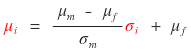
not this

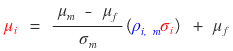
but with the correlation coefficient with the market portfolio

adjusted and plugged in — that’s my conclusion.

This equation is exactly CAPM.

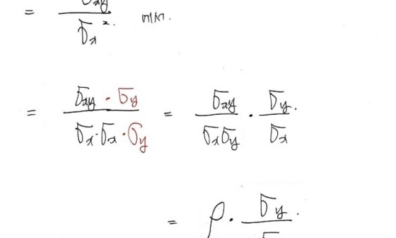
If I tidy the equation up a bit

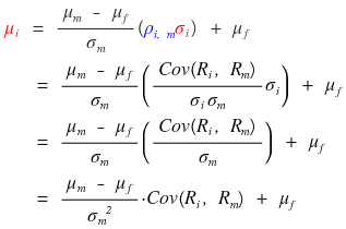
written like this, I feel like I can feel what CAPM is trying to say more directly!!!!

(The notation is wrong. Please read what’s inside Cov as R, not mu!)

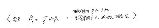
Here I’ll introduce the “stock’s beta”.

The covariance of an individual stock with systemic risk

normalized by this, is called the stock’s beta

they say.

Um then

would be 1, right????????

That is.

can be said to mean “how sensitive is it to systemic risk????” using

as the benchmark

So

This equation from before!!!! This is CAPM, correct, but

when we meet CAPM elsewhere, rather than using this equation,

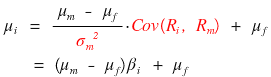
this one is directly used a lot!!!!!

One more thing!!!!

Taking the x-axis as the individual asset’s beta

and the y-axis as the individual asset’s expected return, and drawing the above equation

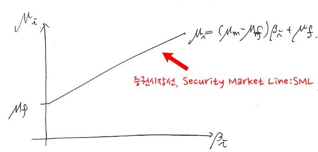
is called 증권시장선 (the Korean name), Security Market Line: SML!!!!!!!!!!!!!!

What does SML mean?????????????????????

With the characteristics of individual stock stock_i

once the sensitivity to the systemic risk that (at the time) exists in the world is determined

the predicted μ_i is linearly proportional to beta

It can also be said like this.

Let’s briefly touch on using CAPM and move on

because apparently there are 2 ways to use this CAPM

so this will be a post that introduces, just roughly, what those two ways are.

The first can be named ’ex-ante CAPM’.

Whether what I have is an individual asset, or a portfolio, or whatever, to use CAPM

for the risk-free interest rate, we can obtain a proxy by using the CD rate, or the government bond rate, or the deposit rate, and so on.

Then the market portfolio….

Above we said we’d substitute with something similar, like S&P500, S&P100, KOSPI 200, KOSDAQ… something like that, right???

That is, find out the relationship (covariance) between the individual asset and that index and use my asset’s return and risk (standard deviation of return)~~~

But you know?

The principle seems… right, and it’s easy enough,

but actually… there can be many cases where it doesn’t make sense…

If someone says those proxies ‘can’t be trusted’, well…. there’s nothing to say

So the second method can be named ’ex-post CAPM’.

Anyway, let’s first organize the use of ex-ante CAPM, where we mobilize any values we can bring in

First

what changed in this equation is that it became p instead of i.

Because we got the conclusion above that we can also predict the return of a portfolio composed of several individual assets, not just an individual asset, I changed it like this.

Then, the values we have to estimate from the values scattered widely in the world total 3 fellas.

The risk-free interest rate,

the expected return of the market portfolio,

the beta of the portfolio I hold

we have to estimate these 3 things,

but as mentioned earlier, for the risk-free interest rate we said to use government bonds or the deposit rate or such things,

and for the expected return of the market portfolio, we said to substitute with the expected return of the composite stock price index.

How do you extract the expected return of the composite stock price index?????

We can calculate it by drawing up scenarios that predict the composite stock price index through a probability distribution, and then computing the expected value of the return with that.

Like this.

Suppose the current stock price index is 1000, and the risk-free interest rate is 2%

Boom

50%

1100

Status quo

30%

1000

Recession

20%

980

Like this — the probability of a boom, the probability of maintaining, the probability of a recession

and if it’s a boom, we expect the index to be 1100, if it’s a recession, we expect it to be 980

let’s say we predict the future like this.

Then next to it, I’ll write out a table that calculates the ‘return (

)’ at each of those times once more in red

Boom

50%

1100

100/1000 = 10%

Status quo

30%

1000

0/1000 = 0%

Recession

20%

980

-20/1000 = -2%

So we can compute the expected return.

Well, something like this?

Then now we also have to estimate the portfolio’s beta value,

if the stocks in the portfolio are stock_1 through stock_n, estimating each stock’s β_i

we have to calculate it like this as the last step.

For now, let’s say there’s only stock A in the portfolio

Stock A’s beta = the portfolio’s beta.

Then the table that contains one’s own predictions for the future of stock A

should be written like this.

Boom

50%

10%

15%

2%

Status quo

30%

0

5%

2%

Recession

20%

-2%

-5%

2%

Looking at this table, we can calculate the ’expected’ return (μ) for each.

This is obvious

this one we calculated before

this one, if you do it, comes out like this

But since we need to find beta, let’s say we’ve found this too.

Now the portfolio’s beta is

ah ah since right now there’s only one stock

can be found like this, rightttt

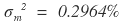
Argh then we also have to find Covariance

But, since we also have a definition for covariance, it’s not that hard a calculation.

Therefore beta is 0.00402 / 0.002964 - 1.356

something like this, we can find it this way.

Having estimated like this

the return of the portfolio containing stock A that I hold is

plugging in and substituting to calculate

= 0.02 + 0.026×(1.356)

= 0.055256

like this, we can calculate it.

Then we can drawww the Securities Market Line

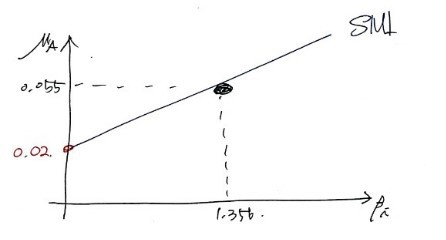
we could draw it like this

and that’s it for ex-ante CAPM

There are people who say the discussions we’ve had before can’t be trusted.

Because the tables about the future…. can’t be trusted…..?

So now the ex-post CAPM story comes up

I’ll take a really light look at how it’s handled.

Ex-post CAPM is about just mobilizing past data that’s come and gone (using a regression model) to inversely estimate the beta value.

Clearly the value β is supposed to represent the ‘sensitivity’ between the market portfolio and my portfolio

so through historical past data, during some period, when

was some value, at those times

was what — pair them up as ordered pairs and then

stamp points like crazy on a coordinate plane like this,

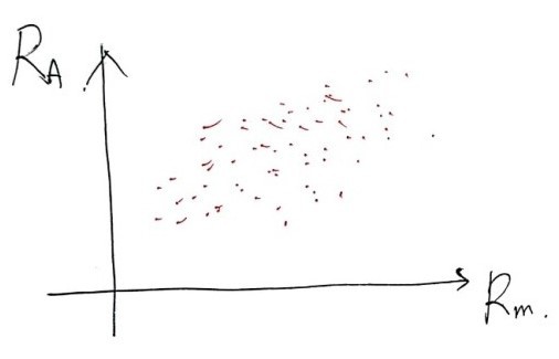
gathering past data and having a look at it

suppose they got plotted like this.

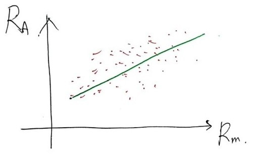
Then (through regression analysis) we pull out one ‘straight line’ where the Error is minimized

and the slope of that extracted line is used directly as the portfolio’s beta.

(http://gdpresent.blog.me/220834860730

The derivatives I studied. Linear regression in the finance field

I thought this would be something I’d need to use as a link in many places, so I pulled it out separately to use just for linking…….

blog.naver.com

In our data, the x-axis is R_m, the y-axis is R_A.

Then if you think of x in the linear regression post as R_m and y in the linear regression post as R_A,

you can confirm that the slope of the green line in the above figure becomes the definition of beta

.)

Suppose we’ve found out the portfolio’s beta like that

we also have to ram in these two things for CAPM to be complete

and this equation

rewritten like this, pulling out a ton of historical risk-free interest rate and excess return data,

estimating the μ_A value, which is the average value of R_A,

(after judging whether using the estimated beta value is reasonable or not~)

ex-post CAPM is completed, is how it goes~

Originally written in Korean on my Naver blog (2016-12). Translated to English for gdpark.blog.