Capital Structure Theory and the Modigliani-Miller Theorem
We break down capital structure theory — from the traditional approach to MM (1958) and modified MM (1963) — and why minimizing WACC is the whole game.
No intro. Diving in.
A company’s capital structure often gets used interchangeably with financial structure, but strictly speaking they’re not the same thing.
Financial structure is about “how and with what funds the money was raised.” Capital structure is about “the composition of the capital the company is actually using.”
OK, let’s go.
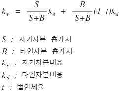
So capital, like we said before, splits into two buckets: equity capital and debt capital.
Equity capital includes common stock, retained earnings, and even preferred stock. Debt capital here is only long-term debt — meaning everything that lands in fixed liabilities on the BS;;.
Why only long-term debt?
Because what companies raise for investment purposes is long-term capital. That’s where our attention is.
The whole motivation behind capital structure theory is this belief that there’s some optimal capital structure out there that maximizes firm value, and finding it is the ultimate goal.
Firm value — we said this last chapter — you take the future cash flows the company is going to receive, discount them at an appropriate rate, sum up the present values, and that’s firm value. And the discount rate? That’s the company’s cost of capital.
And we said the cost of capital we use is the weighted average cost of capital. So firm value $V$ looks like this:
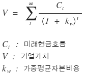
And what this is saying is — the smaller the weighted average cost of capital, the bigger the firm value. Right?
So capital structure theory wants to find the capital structure (how much to hold as $S$, how much to hold as $B$~~~) that minimizes the weighted average cost of capital.
Change the mix of capital, and the weighted average cost of capital can change. Right???
OK so — how do we find the $S$, $B$ that minimize
$$k_{w}$$????????????????
There are three theories about this.
- Traditional capital structure theory
- MM theory (1958)
- Modified MM theory (1963)
I’ll go through them in order.
1. Traditional Capital Structure Theory
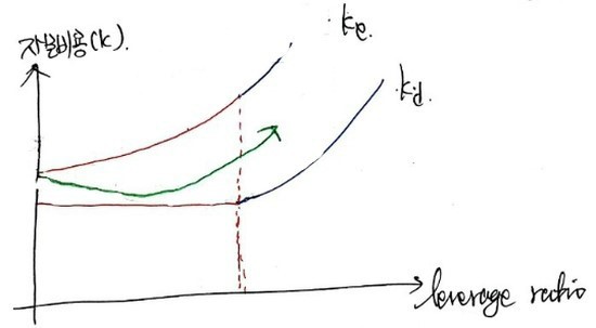
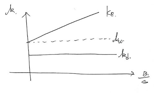
Traditional capital structure theory is actually pretty simple.
Imagine a company with a not-very-high leverage ratio ($B/S$). Even if it nudges that ratio up a liiittle bit, the distrust from outside is gonna stay roughly where it was, right?????
So at low leverage, when the firm cranks the ratio up a tick at a time, the creditors at the existing cost of debt capital

are NOT going to go:
“Hey!!! Where do you think you’re going?!?!?!??!?!!? You little rascals?!?!?!?! If you’re gonna jack up your leverage ratio,

you’d better be paying us a bit more than that.”
So up to some appropriate leverage ratio,

stays roughly flat.
On the other hand,

— that one is not flat.
It rises right alongside the leverage ratio.
That’s because shareholders demand a risk premium.
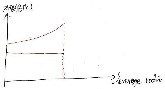
So up to some leverage ratio, for now

stays put,
and

climbs.
But once you blow past that comfortable level, even the creditors start side-eyeing you:
“Hey… you guys are getting a little risky here…..????”
“I think we should be getting a bit more interest….?”
— and they bump up their required return.
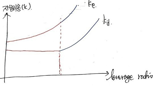
So past that point, both of them are going up.
And now from here,

weighted by each capital ratio,
ends up looking like this:
— that was the academic consensus at the time.
So as you can see, there’s a minimum

(You might be going: WAIT. What?!?!?!?! Why?!?!?!?!
Hang in there for a sec. What this actually means is gonna get unpacked in the MM theory part below.)
That’s the traditional capital structure theory.
But in 1958, a paper dropped that pushed back hard on this — and that’s the MM theory. MM = Modigliani and Miller, the two authors’ initials.
(Technically it’s the Modigliani–Miller theorem. Feels like it should be translated as “MM theorem” rather than “MM theory,” but for whatever reason “MM theory” is what stuck. (sigh))
MM theory (1958)
The setup for the 1958 MM theory is a perfect capital market with no corporate tax.
A perfect capital market means:
- No transaction costs or taxes whatsoever
- Infinite buyers & sellers
- All market info reaches everyone equally
- No constraints or regulations on raising funds (companies can change their capital structure freely, anytime)
Those are the assumptions.
OK, let me walk through what’s called MM’s 1st Proposition.
MM’s 1st Proposition: “In a perfect capital market with no corporate tax, the value of a firm has nothing to do with that firm’s capital structure.”
Firm value is determined by the cash flows flowing into the firm — not by the capital structure. Capital structure is irrelevant.
The classic analogy is the pie.
Picture a firm’s value as a pie. Whether more of this pie goes to shareholders or more goes to creditors — does that make the whole pie bigger or smaller? Flip it around like that and… yeah, kinda nothing to say lol.
But other people pushed back:
“Hey!!! My good sir!!!! What if two companies generating the same cash flows had different firm values — explain THAT!!!!!!?!?!”
To which MM said:
“That’d be an arbitrage opportunity, but since we’re assuming infinite buyers and sellers, that arbitrage opportunity gets eaten up real quick and the market goes back to equilibrium.” (Meaning: whether the stock price goes up or down, it finds equilibrium.)
That’s the MM theory’s pitch.
What does this actually mean? I have no idea either lol lol lol lol.
Let’s go to an example.
Ex. 14.1
Company X and Company Y generate the same cash flows. The table below shows expected cash flows by economic conditions.
Company X has zero debt capital. Company Y has borrowed 1 billion won in debt capital. Interest rate is 10%.
Say Company X’s equity value is 5.5 billion won, and Company Y’s equity value is 5 billion won.

That’s the setup.
Now — since X and Y have the same cash flows, their firm values should be the same!!!!
Hmm, so for X or for Y, the only difference is how much of the same cash flows goes to shareholders and how much to creditors. The total pie going to both groups combined is the same. Right?
So same firm value.
Company X’s equity is 5.5B, and that’s the entire firm value (no debt capital).
But Company Y? Equity 5B + debt 1B = firm value 6B.
In this situation, an arbitrage opportunity opens up.
Say a shareholder holding all of Y’s stock sells all of it, borrows 1B at 10%, and buys all of X’s stock.
Sells for 5B, borrows 1B, buys stock for 5.5B,
and 0.5B is left over????
0.5B in your pocket. And looking at the cash flows that follow:
You’re +0.5B compared to just sitting on Y’s stock?????????????
For there to not be 0.5B sitting in your pocket????
X’s stock price and Y’s stock price would have had to be the same!
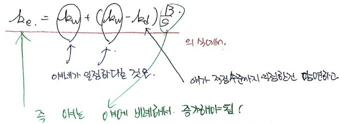
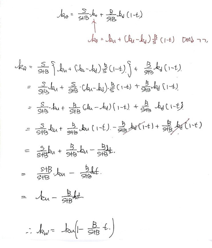
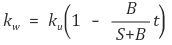
MM’s 2nd Proposition: The cost of equity capital must increase (linearly) in proportion to the debt ratio (leverage ratio).
→ What this means is — in the 1st Proposition,

was constant, right??????
Saying firm value is consistently constant is the same as saying

is consistently constant,
which is the same as saying the 1st Proposition is no different from saying

is constant.

is now under “perfect capital market, no taxes,” so

something like this.
Let me rearrange the equation a different way:
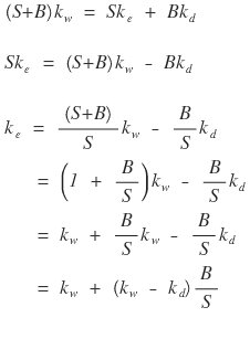
Rearranged like this — interpreting it,
it reads like that.
That is — if

is constant, then

has to be linear, which means
the graph looks like this.
Reading the graph again,
the rise in

precisely cancels out the effect of

falling.
(After hearing this, I started to get a tiny feel for what the traditional capital structure theory was driving at — did you?)
Oh, and the firm value graph — since we kept saying the pie is constant, constant, constant — well, you just draw it like this lol.
But it seems MM kept thinking about this.
And in 1963, they revised the paper and re-did everything assuming corporate tax exists this time — and that’s the modified MM theory.
Modified MM theory (1963)
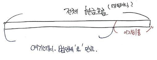
In the no-tax case, the cash flows generated by the firm split between creditors and shareholders.
But when corporate tax shows up!!!!!!!!!
it’s not just two parties anymore!!!!
Shareholders, creditors, AND the government — three parties!!!!!! like that!!!!!
But how is corporate tax assessed??????????????????
If the total cash flow (operating income) looks like the bar above, the corporate tax rate gets applied to the portion after you subtract interest expense.
So from the company’s POV: the more you crank up interest expense, the more you can shrink the slice going out as corporate tax.
Interest expense here is the slice going to creditors (I = the $i$ from chapter 13).
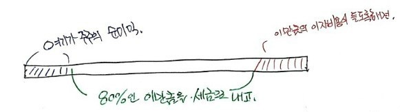
Ahhh~~~~~ if you push this to the extreme — imagine a hypothetical 80% corporate tax rate — you can really feel what’s going on.
If creditors’ slice of the total pie is the shaded portion on the right,
then 80% gets carved out of the unshaded portion, and what’s left is the shareholders’ slice.
The corporate pie was supposed to be shareholders’ slice + creditors’ slice, right?????
So the unshaded portion is gone, and only the shaded portion ends up being the company’s pie.
But this company is fuming. Because it does NOT want to pay taxes!!!
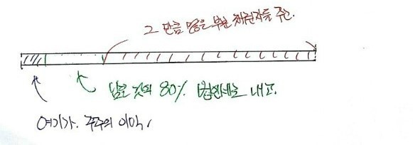
If you crank the debt capital ratio to the max, the money bleeding out as taxes gets cut down. So instead of equity, jack up the debt capital ratio enormously, generate the same operating income, and:

The corporate pie, when corporate tax is in the picture, can change depending on the $S$/$B$ mix.
Let’s put the two bars side by side and compare:
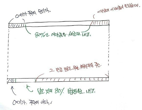
Big difference!!
So this is the tax-saving effect that exists when there’s debt capital vs. when there isn’t.
How do we write this ’tax-saving effect’ as a number?
The firm has to pay out interest expense

as promised on $B$.
From the total cash flow $C$, subtract that interest expense, leaving

then

— $t$ of that gets taken as tax.
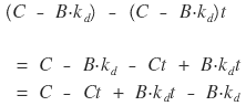
is paid in tax, and the shareholders’ profit left over is
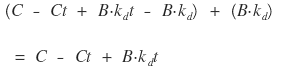
So the firm’s total pie, written as shareholders’ slice + creditors’ slice:

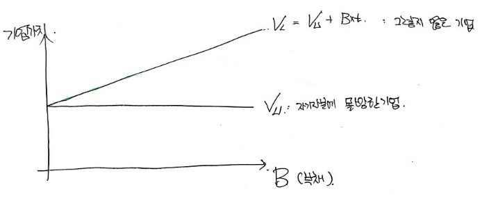
If there’s no $B$ in this picture, plug $B = 0$. Anyway, the firm value in a world with corporate tax for the exact same capital structure but with no $B$ is:

So the tax-saving effect is:

— that’s what it refers to.
But this is the tax-saving effect at the moment cash flow $C$ shows up.
The present value of that is the “tax-saving effect at the current point in time.”
And cash flow $C$ doesn’t happen just once — it keeps happening period after period. So every time $C$ shows up,

a tax-saving effect occurs, and the sum of the present values of every
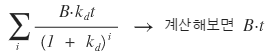
across periods is the “tax-saving effect at the current point in time.”
Written out:

(One more time: this $t$ is the $t$ for tax, not for time (sigh).)
When you actually crunch this (infinite geometric series) — it conveniently shakes out to $Bt$.
The tax-saving effect at the current point in time is $Bt$.
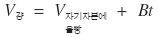
So if a firm running on equity only and a firm also using debt capital of amount $B$ have identical future cash flows, the difference in current firm value is

— and this formula right here is the 1st Proposition of the modified MM theory!!!!!!!
(If you think back carefully, the 1st Proposition of the original MM theory was $V_{\text{plain}} = V_{\text{all-in}}$… heh. You can connect the dots.)
OK now onto the 2nd Proposition… hmm..
The 2nd Proposition in the no-tax case came from playing around with

this equation, so this equation can also be called the 2nd Proposition of the original MM theory.
Let’s say

;
Here, let “corporate pie” be the pie of a firm going all-in on equity. Since it’s also equal to that firm’s pie:
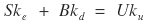
call that the all-in-on-equity firm’s pie.
So:
(plain firm’s shareholders’ slice) + (plain firm’s creditors’ slice) = (all-in-on-equity firm’s shareholders’ slice)
— that’s what the equation was saying. And in the no-tax world this holds, but we now know it doesn’t hold once corporate tax shows up.
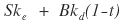
So first, let me write the left side — the plain firm’s shareholders’ slice and the plain firm’s creditors’ slice in a corporate-tax world.
Left side:

Now the right side is where it gets tricky.
In the no-tax world, the shareholders’ slice of an all-in-on-equity firm is:
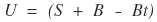
this.
And if we write the firm value $U$ of the all-in-on-equity firm in the no-tax world using $S$ and $B$ from the left side:

— compared to the firm on the left, we tack on $-Bt$ to subtract out the tax-saving effect.
Bottom line: instead of this equation:

the corrected version is:

OK, let’s tidy it up:
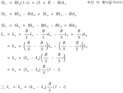

That’s the 2nd Proposition of the modified MM theory~!!!!~~~
There’s also a 3rd Proposition heh.
That equation is, in the corporate-tax case, a relational expression between an all-in-on-equity firm and a not-all-in-on-equity one. And I’ll mash that together with

the formula for the weighted average cost of capital in the corporate-tax case.
Oh honestly, this is;;;; way too tedious to type out….
Sorry lol lol lol lol.
This equation is called the 3rd Proposition of the modified MM theory.
What this equation is saying — it’s packed with the meaning “the weighted average cost of capital decreases in proportion to the debt ratio (debt / total assets = $B/(S+B)$)” ;
and as a graph, that content looks like:
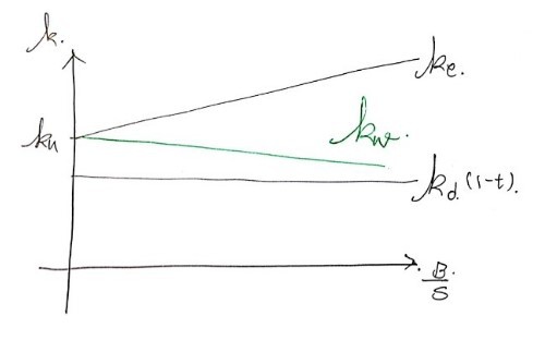
— like this! hehehe.
Drawing it like this, you can capture the whole story.
Which is to say: going 100% all-in on debt capital is the path to maximizing firm value.
And that’s actually where MM theory’s content ends.
But honestly — does that even make sense??????
Are all the great companies in the world right now firms that have gone all-in on debt capital?????
Nope, right?????????????????????
So really, after MM theory, you have to keep extending the theory further and further out.
But of those further extensions, I’m only going to handle one — and not in detail. Pretty much just an intro and then I bail.
The financial management class for 2nd-years at my school ended right here…! hehehe.
(As a dual-major student…. taking a class with 2nd-years when I am as old as a fossil was brutal (sigh)(sigh)(sigh)(sigh) ah…..)
OK OK OK OK OK OK OK OK OK.
Let me draw one more graph about firm value.
This is the graph for this formula:
(Notice the x-axis is $B$.)
Now — as the debt ratio keeps creeping up and up, that gnawing feeling of “ughhhh~~~~~~~~~ I think they’re about to go bankrupt~~~~~~~~~~” gets stronger and stronger, right?????
But say the firm actually does go bust!!!! Just like that.
What happens?
Well, the court decides — rehabilitate or liquidate — whatever’s better, and some follow-up stuff happens. Either way, there’s gonna be a cost.
That cost is called Bankruptcy Cost (I’ll write it as BC. — not B times C.).
So instead of evaluating firm value as:

let’s evaluate it as:
— that’s the idea.
If the firm goes bust, just like that, then from whatever firm value we’d been evaluating, all the BC gets eaten up, and only the rest comes back to us. So if we use the worst-case firm value as our measuring stick,
this equation isn’t totally crazy.
But — how do you actually measure BC…..lol.
How are you supposed to know how much cost you’re gonna incur when the firm goes bankrupt?
So to write the formula above more sensibly,

writing it like this feels more reasonable. (Expected value.)
And this ’expected BC’ — the more debt there is, the more it creeps up, because the probability of going bankrupt is climbing.
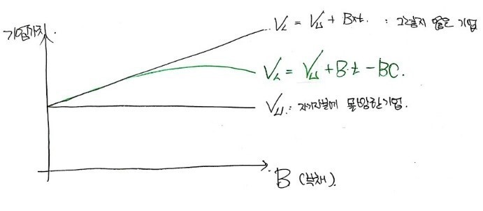
Drawn as a graph, it looks like this??????
Given what I just wrote, the graph isn’t doing anything weird.
That ‘firm value curve’ in the middle? To the best of our knowledge, it’s the most reasonable firm value curve we have.
And that curve has a maximum.
That is — there exists a capital structure that maximizes firm value.
So with that, somewhat abruptly, we slap a period on it —
— and that’s where the major-required financial management class for 2nd-years at my school ended.
It was rumored to be the hardest class at our school lol.
Like a dual-major student would have any business knowing that lol lol lol lol lol lol lol lol lol lol lol lol lol lol.
I just had to take it because the double major required it, and I crammed in whatever fit my schedule (sigh)(sigh)(sigh)(sigh)(sigh)(sigh) ah…..
Anyway anyway anyway anyway anyway anyway anyway anyway anyway.
Financial management this semester was so much fun, and I think I’m gonna go study finance again lol lol lol lol lol lol lol lol lol lol lol lol lol lol lol lol lol lol lol lol.
I’m REALLY never doing this again lol lol lol lol lol lol lol lol lol lol lol lol lol lol lol lol lol lol lol lol lol lol lol.
It’s so damn hard for real;;;;;;;;;;;;;;;;;;;;;;;;;;;;;;;;;;(sigh)(sigh)(sigh)(sigh)(sigh)(sigh)(sigh)(sigh)(sigh)(sigh)(sigh)(sigh)(sigh)(sigh)(sigh)(sigh)(sigh)(sigh)(sigh)(sigh)(sigh)(sigh)(sigh)(sigh)(sigh)(sigh)(sigh)
Originally written in Korean on my Naver blog (2016-12). Translated to English for gdpark.blog.