Linear Regression in Finance

I figured I’d be linking back to this thing constantly down the road,

so let me just pull it out into its own post and treat it as the canonical link… heh heh heh heh.

Today’s quick(?) topic: linear regression, which gets used all the time in finance.

I really don’t like just hurling formulas at you and saying “here, use it.” Feels gross. But the further we go, the more formulas pile up, and deriving every single one in real-time is… yeah, not gonna happen.

So I’m gonna derive this one, just this once.

Because it’s important. Not just for finance — this thing shows up everywhere in the real world!

OK so, simply put, what is linear regression even trying to do?

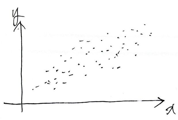
Say you’ve got a pile of data plotted like that.

You want a line that captures these points well enough that you can guess what happens at a bigger $x$, or a smaller $x$, or wherever.

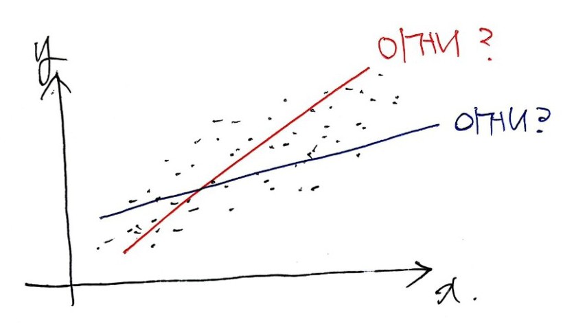
Which one of these is it??

But — a straight line.

(Fitting a curve? That’s for next time ^^)

Fitting a straight line has one really, really nice property.

That property is something you pick up in linear algebra… so I’ll skip going into it here.

(Apparently the reason mathematicians make such a big deal about the linear/nonlinear split is exactly because of that property.)

The other thing is — nonlinear is brutally hard. So linear it is!!

OK. Which straight line best represents the data?

Aaaand what’s our criterion for “best represents”?!?!?

Error. Obviously.

The line that makes the error as small as possible —

that’s the one we want.

Lucky for us, a straight line is fully described by just two things: its slope and its y-intercept. So we just need to find the slope (square) and the y-intercept (triangle) that minimize the error.

Now, how do we handle that error?

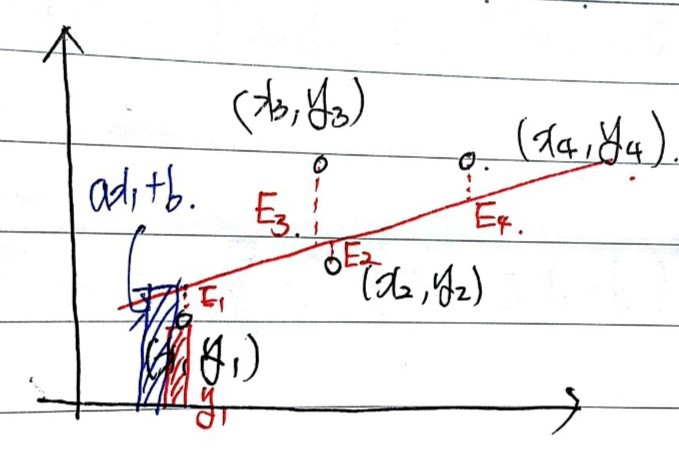
Say the black dots are our data points.

We want $y = ax + b$ that best represents them — meaning we want to find $a$ and $b$.

Suppose that red line is the best one. Then the errors are $E_1$ through $E_4$ as drawn above.

To minimize these errors, do we just find $a, b$ that minimize $E_1 + E_2 + E_3 + E_4$?!

BZZT. Wrong.

We need the $a, b$ that minimize the sum of the squares of each one.

(Why? The $a, b$ minimizing the plain linear sum of $E_i$ aren’t unique — kind of awkward to explain in one breath, but think back to high school stats: when you want variance — how spread out the data is — you don’t take the average of distances from the mean, you take the average of the squares of those distances, right? Same deal here.)

So now we’ve got a real, quantifiable error, right??

Yep~~~~~

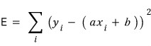
Let’s write out the sum.

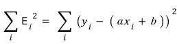
I’ll call this sum-of-squares thing big $E$.

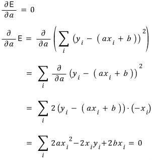
Now: how do we find the $a, b$ that minimize $E$?

Treat $E$ as a two-variable function in $a$ and $b$.

The minimum is gonna be at an extremum, so we partial-differentiate $E$ with respect to $a$, and partial-differentiate with respect to $b$,

and find the $a, b$ where both partial derivatives are zero.

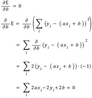
And the partial derivative with respect to $b$ set to zero:

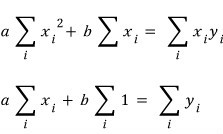
So the two equations $a, b$ have to satisfy are

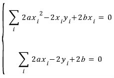
exactly these two, and

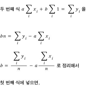
cleaning them up a bit,

Oho. Now let’s solve these two simultaneously to pin down the $a, b$ that satisfy both at once.

(Naver’s equation editor, please wake up and become a tool that’s actually pleasant to use. Improve!! Improve!!!)

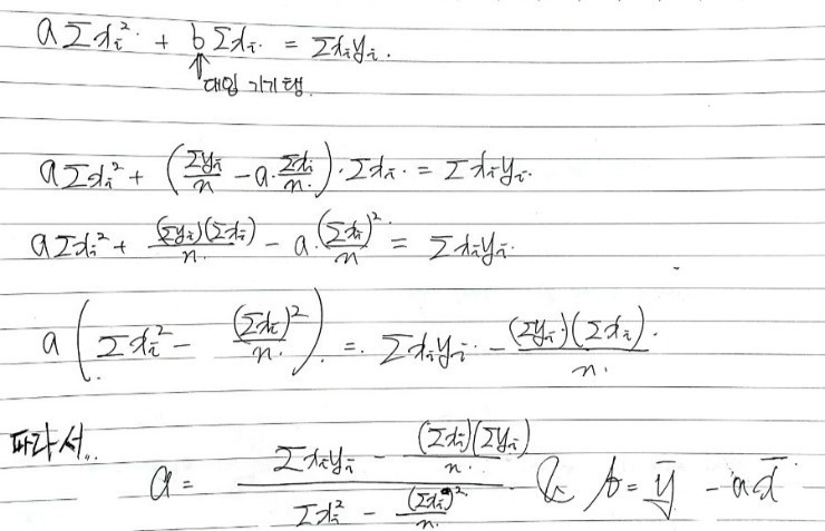
And just like that — kinda anticlimactically — the hunt for $a, b$ is over. But let me massage $a$ into a more interesting form,

because I want to mess around a little more.

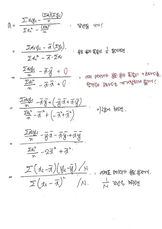
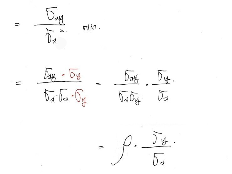
Looking at the data,

the slope $a$ of the best-fit linear curve — that $a$ —

is exactly

We made it!!!!

Oh, one thing I skipped — that $\rho$ in there is the correlation coefficient.

Anything else I forgot to flag?

That right there is the covariance!! That one too!!!

Covariance is a statistically defined thing, and from it the correlation coefficient gets defined as a consequence!!

What does the correlation coefficient actually mean? I went into that elsewhere —

My study of basic investment theory #10: Diversification

In the previous post we set up a risk-free portfolio F and a risky portfolio P, and then inside that risky portfolio P…

OK, but here:

• $x$ is $\Delta F$: the change in futures price over the hedge period
• $y$ is $\Delta S$: the change in spot price over the hedge period

So if we call the minimum-variance hedge ratio $h^\star$, it’s defined as

like that.

And if you think about it for a sec,

it kinda makes sense that $h^\star$ is defined

this way.

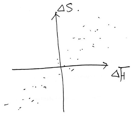
Like this — over some time window, we plot the historical $\Delta F$ vs $\Delta S$ as points,

fit the best straight line,

and use the slope of that line as our hedge ratio!

So when there’s some amount of change in the futures price, the spot price moves roughly by this much,

and then the correlation coefficient grabs hold of how tight that relationship actually is, one more time,

and we hedge that amount!

So — if the spot price changes by 4, factoring in the correlation, the corresponding futures change works out to 2, and since spot moves by 4, we defend that 4 using the futures!!

Yeah, something like that… (I’m kinda just tossing this out, and I’m a little nervous it might actually muddy the concept rather than clear it up.)

And since we need to defend the same quantity for that amount,

we now scale to $h^\star$ by accounting for contract size.

That is, the optimal number of futures contracts is

• $N^\star$: number of futures contracts for the optimal hedge
• $Q_F$: size of one futures contract
• $Q_A$: size of the position being hedged

Originally written in Korean on my Naver blog (2016-10). Translated to English for gdpark.blog.