Properties of Stock Options
Breaking down every variable that moves option prices — S, K, T, σ, r, and D — and why European vs. American options handle time to expiration differently.
OK heads up — this one’s a wall of text. Like, insane wall of text. The practice problems? Saving those for the next post.
Today we’re looking at the things that move stock option prices, comparing European vs. American options, and then heading toward put-call parity.
Let’s dive in.
What moves an option price?
The variables in our model:
- $S_0$ — current stock price
- $K$ — strike price
- $T$ — time to expiration
- $\sigma$ — volatility
- $r$ — risk-free rate
- $D$ — dividends
Compared to just thinking about the stock by itself, we’re now thinking about the option on the stock, so naturally $S_0$, $K$, $T$ all show up in the mix.
So — what’s the sign of the relationship between each of these and $c, p, C, P$? (lowercase = European, uppercase = American.)
Let me just dump the whole table first:
| $c$ | $p$ | $C$ | $P$ | |
|---|---|---|---|---|
| ① $S$ | + | − | + | − |
| ② $K$ | − | + | − | + |
| ③ $T$ | ? | ? | + | + |
| ④ $\sigma$ | + | + | + | + |
| ⑤ $r$ | + | − | + | − |
| ⑥ $D$ | − | + | − | + |
Honestly I wanted to just slap a photo of this table down and call it a day, because typing it all out is so much work. But fine. Fine. Let’s go through each row.
① $S$ vs. option price. If you imagine the stock price going up, like, a lot… it might not click immediately. So let me put it differently. Imagine it goes up insanely. Like ridiculously, absurdly through the roof.
Anyone holding a call goes nuts. “OH YEAH, MASSIVE GAINS!!” Trigger the call, buy at the low strike, resell at the moonshot price~~
Meanwhile, anyone holding a put is over there like “ugh, my prediction was so off T_T T_T T_T.”
So $S$ vs. $c$ is (+), $S$ vs. $p$ is (−). Same logic obviously holds for $C$ and $P$ where you can early-exercise.
② $K$ vs. option price. Say you’re shopping for a call, and there’s one with a crazy high strike. The chance of it ever being worth exercising is basically zero. Who’s buying that? Nobody. So high $K$ → low $c$.
For a put, on the other hand, a high $K$ means it’s very likely to be exercised in your favor. That should be priced expensively, right? So high $K$ → high $p$.
So $c$ vs. $K$ is (−), $p$ vs. $K$ is (+). Same logic for American — early exercise doesn’t change this.
③ $T$ vs. option price. This is actually the one most affected by early-exercise rights.
For all the other variables, the European/American distinction didn’t matter. But for $T$ it does.
For $C$ and $P$ (early exercise allowed): more time = more value. $T\uparrow \Rightarrow C\uparrow, P\uparrow$. Easy.
But for $c$ and $p$ I wrote “?”. The “?” means sometimes (+), sometimes (−).
Generally yeah, more $T$ means more $c$ and more $p$. But —
For the call: imagine you stretch $T$ out, and somewhere in that extra stretch, suddenly a dividend payment date falls inside the window. Painful, right? Exercising the call after the dividend has been paid out feels gut-wrenching. So as $T$ creeps up, snap — the call value can actually drop.
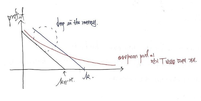
For the put: apparently if you plot put value vs. $T$ using Black-Scholes, in deep in-the-money scenarios, you can see the put value actually decrease as $T$ grows. (I’ll write a little program later that lets you verify this — I’ll share it.)
So the conclusion: for $c$ it’s dividends, for $p$ it’s the BS formula behaving weird ITM. Either way, you can’t make a clean blanket statement about how $c$ and $p$ move with $T$.
④ $\sigma$ vs. option price. Higher volatility means the stock could rip or tank — both possibilities are now bigger. But why is the table all (+)? Because options have no downside risk. That one sentence should do it. If not, sit with it for a sec.
⑤ $r$ vs. option price. Imagine the risk-free rate is insanely high. (If that doesn’t click — picture bank deposit rates being absurdly high.)
You and I agreed I’d buy at $K = \$10$. But if $r$ is sky-high, the present value of that future $$10$ is basically garbage. Trash.
So a rise in $r$ effectively makes the strike feel like garbage. When you trigger a call and pay $K$, having that $K$ feel like garbage is good for you — so the call price should go up. Triggering a put and receiving $K$ — that $K$ now being garbage is bad for you — so the put price should go down.
That’s why row ⑤ has those signs.
⑥ $D$ vs. option price. Suppose dividends balloon (and remember, options generally don’t adjust for dividends). You buy at the same agreed $K$, and the person who got called on — the stockholder — is sitting there going “oh yeah baby, I cashed those fat dividends~~”, while the person who exercised the call is going “you S.O.B… I want my stock back T_T T_T.”
That feels bad, doesn’t it? Which means call value drops. (If you feel bad, you just lower the price you’re willing to pay for the call, lol — prices are set by supply and demand anyway.)
For the put, flip the reasoning. I’m not gonna re-type it all out — that’s what I wrote back then, heh.
Setting up for put-call parity
OK from here we’re slowly, slowly, slowly tightening up the conditions for option pricing. The destination: put-call parity.
To get there, let’s lay out our assumptions:
- No transaction costs.
- All trading profits taxed at the same rate.
- We can borrow and lend at the risk-free rate.
- If an arbitrage opportunity appears, it’s instantly snapped up → i.e. no arbitrage.
With those locked in, let’s see what basic rules fall out.
Upper and lower bounds on option prices
Options necessarily have an upper and a lower bound on their price. Why??????
Because outside that range, there’d be an arbitrage opportunity. The “no-arbitrage range” is the bounded range of allowable option prices. (Outside the bounds = arbitrage exists.)
Sounds grand, but it’s actually pretty simple. T_T
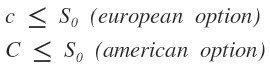
If the call price went above this upper bound? People would buy the underlying and short the call — locked-in profit, immediately.
(If you can sell a call for 600 when the underlying is at 500, then even if the buyer exercises, you just hand over the stock — boom, +100 locked in.)
So that upper bound gets enforced by arbitrageurs.
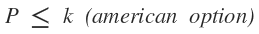
For the American put, $P$ has to be greater than $K$. No matter what. Because you can exercise at any time — if the option price exceeded $K$, you could just sell the put for more than $K$ and instantly profit.
(If you can sell a put with $K=500$ for 600, you got 600 in hand, and if the buyer demands to sell at 500, you fork over 500 — net +100. Such a thing doesn’t exist in this world, lol.)
So:
And for the European put:
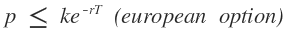
The price has to live in this range. Same reasoning — if the inequality flipped, you’d sell the put, grow the proceeds at $r$, end up with $p\cdot e^{rT}$ at maturity, only owe $K\cdot e^{rT}$, and pocket the difference. Arbitrage. So that gets enforced too.
That’s the upper bounds.
Now the lower bounds.
The whole logic is one thing: no arbitrage.
Concrete example. Say $S_0 = 20$, $r = 10\%$, $T = 1$ year. Find the lower bound on the European call with $K = 18$.
In other words: what’s the minimum $c$ such that no arbitrage exists?
Strategy: short-sell one share, pocket $S_0 = 20$. We’re going to need to buy the stock back later to cover the short, so let’s also buy one call at $K = 18$. Call costs $x$ (unknown).
Cash in hand right now: $20 - x$.
Grow it at the risk-free rate. After 1 year:

Now exercise the call. Pay out $K = 18$. Cash remaining:
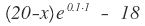
For no arbitrage, that remainder has to be 0 (anything positive would be free money). So solve:
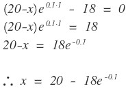
That $x$ is the no-arbitrage point. If instead
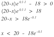
we’d have arbitrage. So the no-arbitrage condition is:
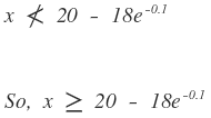
That’s the lower bound for the European call. Rewriting the numbers back as symbols:
There we go.
Now the European put lower bound. Same logic, one thing: no arbitrage.
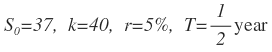
Try this. Borrow $\$37 + $x$ at the risk-free rate to buy a $$37$ stock. (From here on I'll drop the $$$ and just write numbers.)
Drill into your head ahead of time: the amount we owe after 6 months is
Buy 1 stock at 37, and to lock in selling it for 40 at maturity, simultaneously buy a put.
How much cash do I have right now?? Zero. Nada.
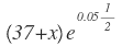
At maturity I trigger the put, sell the stock for 40, so I now have 40 in hand.
Out of that 40, I owe:

Net cash remaining:
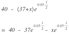
That’s the arbitrage profit. For no arbitrage, it has to be 0:
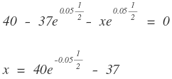
That’s the minimum put price. If
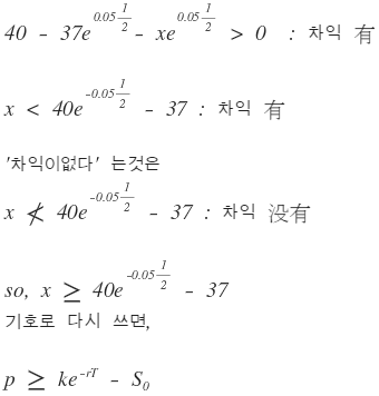
— that’s where arbitrage exists.
Done. We’ve got the lower bound for European puts too.
At least this much, or arbitrage exists!!
But wait — what if the lower bound comes out negative?
We learned in a previous chapter that an option’s value is always $\geq 0$. So an inequality saying “price > some negative number” would technically allow negative prices, which is nonsense.
To make it cleaner, we write the lower bound like:
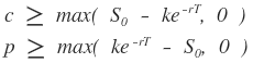
i.e. “max with zero.”
Put-call parity
Upper bounds, done. Lower bounds, done. Now let’s pull one equation out of all this.
Because between a call and a put with the same maturity, same strike, same underlying — there’s a rule.
Why is there a rule???
Because of that one logic: no arbitrage.
This can be drawn out as a single graph all at once, but I want to talk through the scenario first and then nail it with formulas.
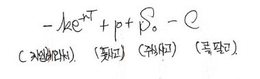
We’re constructing a risk-free portfolio. Here’s the recipe:
First, borrow money

at $r$ (= sell a zero-coupon bond), buy a put, buy the stock. And sell one call. Done — risk-free portfolio.
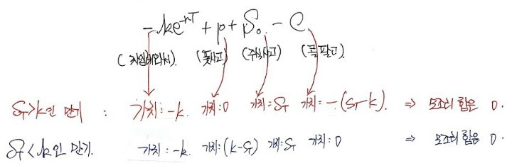
Why?
Case 1: stock ends above $K$.
The person who bought our call is going wild: “Yes! Buying at $K$~~ hand over the stock please~~”
We hand over the stock, receive $K$.
What we borrowed —

— has to be repaid as $K$. So we just hand them the $K$ we just received from the call buyer.
The put we’re holding? Worthless.
Started with empty hands, ended with empty hands. (Empty in, empty out → no arbitrage.)
Case 2: stock ends below $K$.
The call buyer stays quiet. We exercise our put — sell the stock for $K$.
Hand over the stock, receive $K$, repay the $K$ we owe. Empty in, empty out again.
So whether the stock ends above or below $K$, we end with zero. Always zero.
Lives up to the name “risk-free portfolio.”
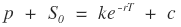
Now let’s nail it with formulas.
At $t = 0$:
Our position value, which was this, becomes:
in each scenario at maturity.
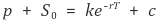
Equivalently, set the initial value to 0:
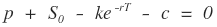

This is the relationship between put and call!!!
We can run the reverse construction too.
Again, start empty-handed. Borrow a stock and short it. Sell a put. Buy a call. And —

— lend the cash at $r$.
At maturity, if stock ends above $K$:
What we lent out —

— has grown to $K$. We receive $K$.
We use that $K$ to exercise the call, get the stock, use the stock to close the short. Left with??? Zero. Empty in, empty out.
If stock ends below $K$:
The call we hold is worthless.
The put buyer is going wild demanding to sell at $K$. With the $K$ we get back from our loan, we pay them, receive the stock, and use it to close the short. Empty in, empty out, again.
So once again:
If this didn’t hold? Then it’s not empty-in-empty-out → arbitrage exists.
So $c$ and $p$ (European, same maturity, same strike) must always satisfy this. That equation is put-call parity.
What about American options?
Above I was subtly stressing “European.” That’s because for American options, you don’t get a clean equality between put and call.
You can, however, derive an inequality:

Let’s see how.
Look at the right side first. Why does the max work out like that?
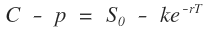
European put-call parity says:
How does this become an inequality…?
For American options, you have to internalize: early exercise is not always optimal.
For a call on a non-dividend-paying stock, early exercise is actively worse.
European call value with $T$ remaining:

For the American version, if you just sit there, you get the same value. But the moment you early-exercise:

— smaller.
($K e^{-rT} < K$, and when you subtract a smaller number, the result is larger. So sitting still gives the larger value.)
So early-exercise value is worse. (This story changes when there are dividends — you grab the stock early to collect the divs — which is why I keep emphasizing “no dividends.”)
So for no-dividend stocks, the best-case value of a call is the same whether European or American!
In other words:
So the formula:
can be rewritten that way without loss.
But for puts, early exercise can be advantageous.
Same method as above. European put value with $T$ remaining:
American value if you sit still: same thing. But if you early-exercise immediately:

— larger.
(To be precise, it’s not strictly always larger — there’s time value to think about — but there are real cases where early exercise wins. The picture below should make this click.)
So for the no-dividend case:
That accounts for the right side of the inequality.
(Why does the equality become a “smaller-than”? Just look at the left side. We were subtracting $-p$, but now we’re subtracting the larger $-P$ — so a crack opens up in what was an equality. Left side gets smaller.)
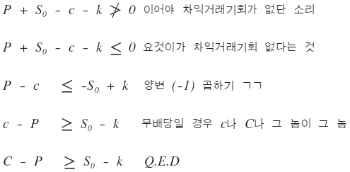
OK now:

let’s prove the left side.
Why does early exercise have to give us at least that much?
Since calls don’t differ in the no-dividend case, we can put $C$ aside and focus on the put.
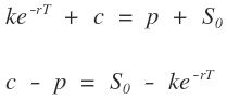
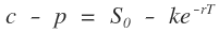
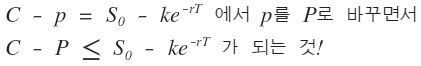
Back to put-call parity:

This was originally derived by constructing a risk-free portfolio. But now let’s think of the put as American, not European:
(Capital $P$.) Is this still a risk-free portfolio?
I don’t think so.
Because if we trigger $P$ right this instant —
we sell the stock now for $K$, hand over the stock, receive $K$ on the spot. Then instead of paying back $K$ at maturity, we only need to repay:

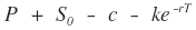
So an immediate profit of:

pops out, right?
That’s an arbitrage opportunity.
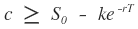
So for American options, to actually be risk-free, we need:
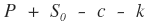
Therefore:
So putting it all together:
European case:
American case:

Should I name this thing? Just call it “American inequality”? lol. Anyway.
Bringing dividends back in
But — the no-dividend assumption was baked into all of the above!
Now suppose dividends do show up, and we know when and how much in advance.
(cf. Most exchange-traded options have maturities under 1 year, so the “dividends are known” assumption isn’t unreasonable.)
Let $D$ = present value of the dividends.
For European options, fixing parity is easy: just replace $S$ with $S - D$.
Why? Because shareholders are gonna show up like “hey you stockholder! Cough up the divs!!”, and $S$ drops to $S - D$.
If that didn’t happen, the stockholder would pocket a guaranteed instant gain — which violates no-arbitrage. There can’t be a guaranteed immediate profit.
So:

becomes:

That’s put-call parity with dividends.
Now revise the inequality.
The right side doesn’t need fixing. The maximum occurs at $D = 0$ (assuming the put gets exercised at maturity — if it doesn’t, the inequality holds trivially anyway). And as $D$ grows in the (+) direction, the inequality slack just widens.
So:

That’s fine. The piece that needs fixing is the minimum.
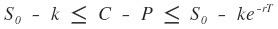
The minimum of $C - P$: now that $D$ is in play, $C$ shrinks and $P$ grows, so the minimum has room to drop further. Specifically, the new minimum is $S - K - D$:

And that is the American inequality with dividends.
OK seriously, this wall of text is insane. The related practice problems are going in the next post.
Originally written in Korean on my Naver blog (2016-11). Translated to English for gdpark.blog.