Options Trading Strategies (Part 1): Spreads — Bull Spread, Bear Spread, Box Spread, Butterfly Spread, Calendar Spread
We finally stop staring at one lonely option and start building real portfolios — covered calls, protective puts, and every spread you'd want to know.
Up to now we’ve been looking at exactly one option. Just one, naked and alone.
So now that we know the personality of a single option — what its payoff looks like, how it behaves — the natural next question is: OK, so how do we actually use these things?
That’s basically what this post is about. We’re going to look at the special portfolios you can build out of options. And these portfolios fall into roughly 4 buckets:
- Option + zero-coupon bond
- Option + underlying asset (a stock, here)
- Two or more options of the same kind → Spread
- Two or more options of different kinds → Combination
OK let’s go.
So first — if you have some money and a zero-coupon bond, what kind of security can you cook up?
A “principal-guaranteed product.” Right there, on the spot.
But this one is kind of… too obvious. Like, the logic is:
A zero-coupon bond pays exactly its face value at maturity, right? So if you “invest” only as much as that face value — which you’ll get back 100% (assuming no default) — then yeah, by definition you’ll get your principal back. Boom, “principal-guaranteed.”
But hold on. If I put in 100 and three years later the world has gone to hell, but I still get 100 back because it’s principal-guaranteed… I haven’t lost or gained anything?
NO NO !!!! Putting in 100 and getting 100 back three years later is a loss. I should’ve at least made the risk-free rate. Why am I getting it back as-is? What is this, a piggy bank?
OK so. Something with face value 100 obviously can’t be sold for 100 three years before maturity. Let’s say it’s discounted and you buy it for 80. Then you stick the remaining 20 into options. Total investment: 100. Right?
At maturity the bond pays 100 face value, and since 100 was your invested amount, that’s what “principal-guaranteed” means. (OK I actually get it now.)
Worst case → principal is intact. Any upside comes not from the bond but from the option side.
Anyway, that’s enough on this one. Let’s move on. The stuff I actually want to dig into here is #2, #3, and #4 — well, #3 and #4 mostly.
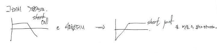
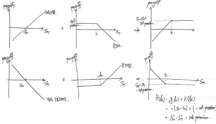
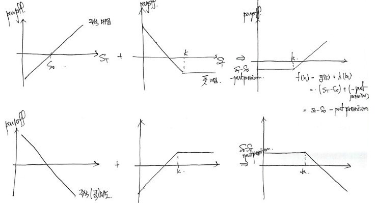
Stock + option
By name: covered call and protective put.
I mentioned before that the meaning of “naked option” really clicks here. The non-naked situation isn’t an option standing alone — it’s an option covered or protected by some stock! That’s what those names are doing, you jerk.
OK from here on I’m going to express everything… in graphs.
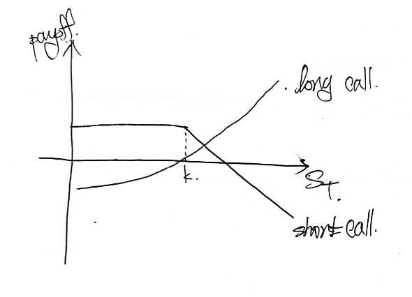
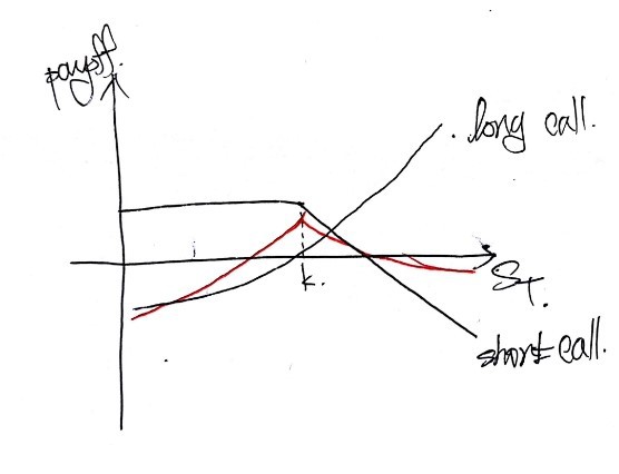
Let’s say the portfolio is: buy a stock + sell a call (same underlying, obviously).
Draw the payoff against the stock price for each leg:
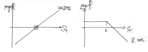
(On the left graph, the $S_T$-intercept is $S_0$, but I didn’t label it… you know that, right? heh haha)
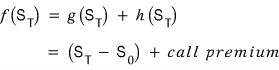
Each leg drawn separately looks like that. The portfolio has both, so the portfolio payoff is the sum of those two graphs (because the underlying is the same):
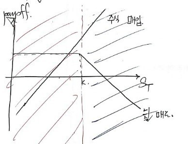
I’d love to just sum them in one shot, but the option payoff is nonlinear, so I can’t naively do $f(x) = g(x) + h(x)$. Need to split the domain a bit and then sum piecewise.
Lucky for us, both legs have slope 1 with respect to $S_T$, so this is easy. Very easy.
In the picture above, on the left side — the red region (you can’t see the color, sorry) — taking $S_T = k$ as the cutoff, the summed slope is 1. To the right of that (blue region), the summed slope is 0.
So it ends up looking like this!
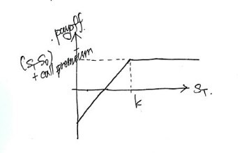
(I don’t know if everything I want to say is going to come through in just words, but let me try. In the red region, the portfolio payoff is the original “buy stock” graph shifted up by +call premium. In the second region the slope is 0, so it’s a horizontal line — but at what level? How do we find that?)
That’s why I wrote the levels like that;; heh heh heh
Yeah. That’s what I was just going on about.
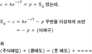
And the reason $S - c = p$? You can also confirm it from put-call parity.
OK then — the long and short payoffs of a covered call (which looks like a put built out of stock + call), and the long and short payoffs of a protective put (which looks like a call built out of stock + put) — let me just slap them all up at once and wrap this section.
Now the question that probably popped into your head: why bundle a stock with an option to fake a put or a call? Why not just buy or sell a put or a call directly?
Hmm… lots of reasons, but here’s one: before going out and buying a fresh option, you can use options you already hold to synthesize a different one. Something like that.
Now — spread. The portfolio you build by combining 2 options of the same kind.
We’re going to look at 6 of these:
Bull spread, bear spread, box spread, butterfly spread, calendar spread.
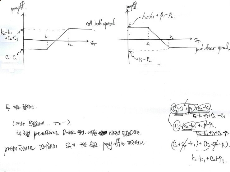
① Bull Spread
Apparently one of the most-used spread techniques out there.
Two options of the same kind. How are they different? Like this:
Buy the option with the (relatively) lower strike & sell the option with the higher strike.
That’s the combination. (Same maturity, same underlying, obviously.)
Draw the payoff at maturity for each on the same axes:
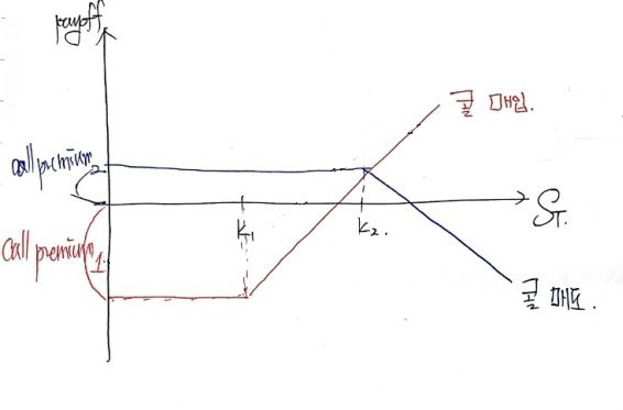
Same kind, so let’s say both are calls. I bought the lower-$k$ call and sold the higher-$k$ call.
Now do the function sum:
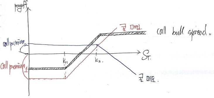
Anyone object that it comes out like this? Anyone?? Obvious, right???
But there’s one thing here that’s not obvious — I drew the price of $\text{call}_1$ as bigger and $\text{call}_2$ as smaller, kind of out of nowhere. Hmm. But this is actually true.
Why? Because the lower the strike, the higher the call premium. Obvious!
(For anyone who’s just dropping in, quick gut-check: imagine selling someone the right to buy a pen GD park used for 25 million won. How much would that cost? haha. Yeah. Now it clicks, right?)
OK so. In the picture above, there are flat horizontal segments and I haven’t said what level they’re at. Let’s figure that out.
Plug $k_1$ and $k_2$ into the bull spread function and you get the upper and lower bound levels of the payoff.
Real talk, please bear with me today; typing this stuff in the equation editor is such a pain. I’ll come back later and replace the patched-in photos with proper formula-editor versions, promise.
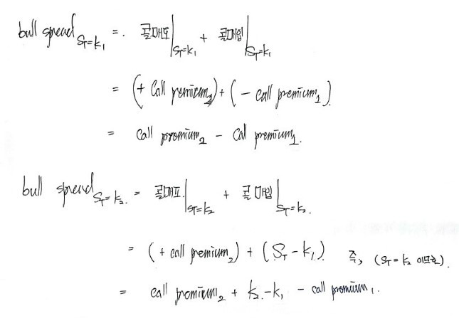
(Second-to-last line from the bottom — under the formula — I forgot to write $-\text{call premium}_1$… T_T T_T T_T)
Can you read it OK??
So that’s the upper and lower bound. And what about when

is between

and

?
Since we haven’t substituted

yet, we just leave it as

heh heh heh
OK let’s do the same buy-low-strike & sell-high-strike thing but with puts this time.
Out of two puts, buy the lower-$k$ one, sell the higher-$k$ one. And without overthinking it, just draw both payoffs at maturity on the same axes.
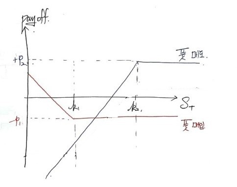
I just bought and sold the puts as instructed, no thinking.
(Same underlying, same maturity, obviously… I’m so tired of saying this T_T T_T T_T)
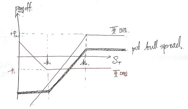
Slam them together as a function sum and the picture comes out like this. Anyone object?? Obvious, right?!?!
And we coolly write “put bull spread” next to it and we’re done. heh heh hahaha
What about the premium sizes? The right to sell a pack of ramen for 50 million won — cheap or expensive??? Since there’s basically zero chance it ever gets exercised, it’d be insanely expensive. So the higher-$k$ put gets drawn as the more expensive one!
Now — same as before, let’s nail down the upper and lower bounds of the put bull spread. This should be quick.
Starting from

work it out:
And what about when

In the middle?!?!?!
In the middle, we still haven’t substituted those conditions in, so
that’ll be it, I guess~~
② Bear Spread
Bear is the opposite of bull.
Position: buy the higher-strike option & sell the lower-strike option. For this one too — without thinking — let’s start with calls. Sell the lower-$k$ call, buy the higher-$k$ call. Stack their payoffs on one set of axes:
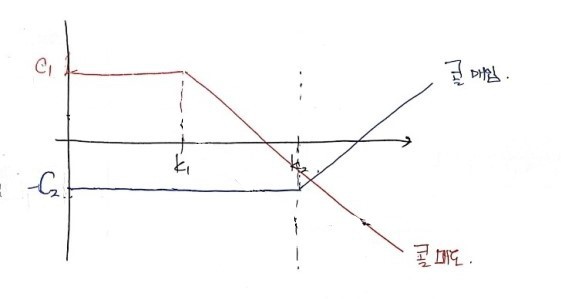
Yeah, looks something like that. Same logic: the right to buy at a lower strike has to be more expensive, so $c_1 > c_2$.
And now slam them together as a function sum, no thinking required. (Try it yourself;)
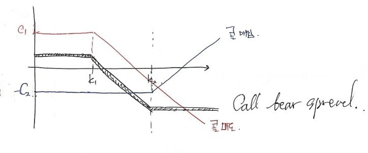
Anyone object?!?!? Good good good.
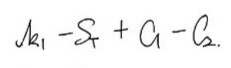
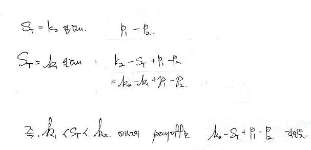
OK now the bounds. This time I’ll just write the formulas:
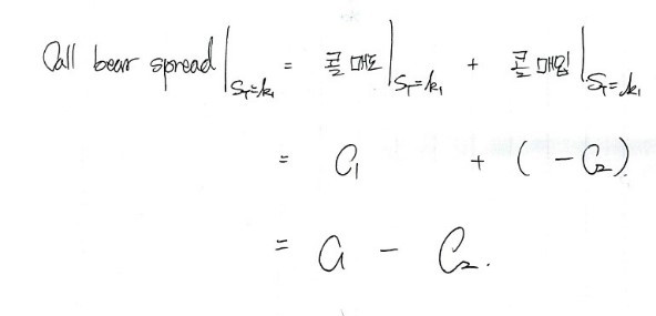
Upper bound~~
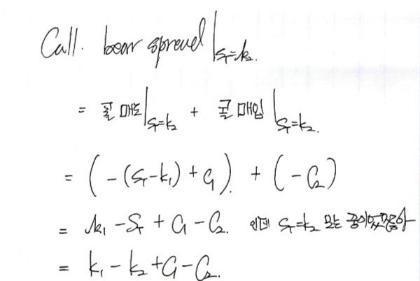
Lower bound~~~
And here’s how the linear segment in the middle is derived:
Just — this is before substituting $k_2$ for $S_T$~~
Now play with puts, why not?!
Don’t forget: bear spread is buy high-strike & sell low-strike!
This time I’ll cram everything into one picture:
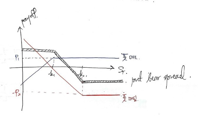
Like that!
And once you nail down each segment:
Smooth sailing~~~~ Was that too easygoing???
③ Box Spread
What’s a box spread!!
Simple!
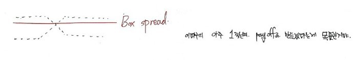
Easy, right!
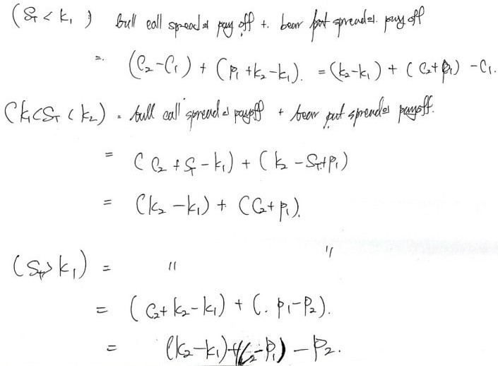
But the catch — you have to combine call bull + put bear. Combining put bull + call bear is useless.
Why? If you combine those, the flat-line payoff comes out negative. Lower $k_1$ → call gets more expensive, put gets cheaper. That’s the property we just used. And that property is exactly what flips the sign.
So a box spread is only call bull + put bear. Period.
Let’s pull in the call bull spread and put bear spread we drew earlier:
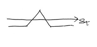
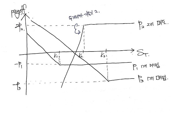
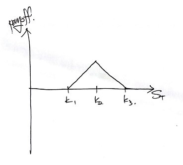
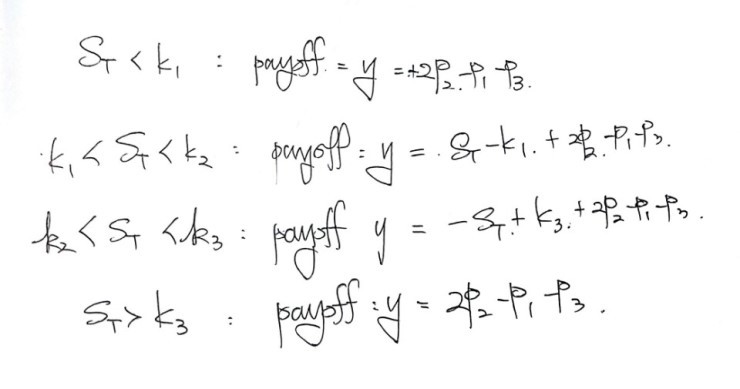
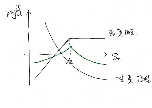
④ Butterfly Spread
Bull, bear, box from before needed 2, 2, and 4 options respectively, but only two strikes ($k_1, k_2$).
Butterfly needs three strikes ($k_1, k_2, k_3$) and uses 2 — wait, no, it’s still spread, so same kind of options — and uses 4 of them. Let’s go!
with the condition
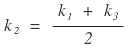
attached. So $k_2$ has to sit at the midpoint.
Let the call premiums be $c_1, c_2, c_3$.
(Lower strike → more expensive call, so $c_1 > c_2 > c_3$.)
Recipe: buy 1 of $c_1$, sell 2 of $c_2$, buy 1 of $c_3$.
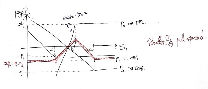
4 calls total = butterfly. Stack the payoffs at maturity on one set of axes:
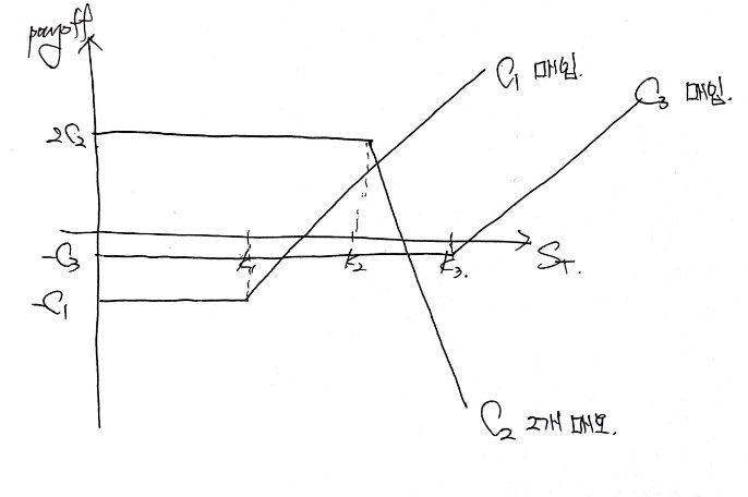
There it is.
Drawn this way, it’s pretty easy to picture the sum of the three:
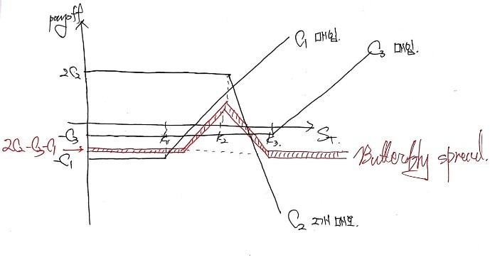
And as for why it comes out like this:
think of it that way and it’s straightforward.
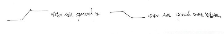
But hold on!!
I drew it so that everything is below the x-axis and only that one boing! part pokes up into positive territory.
Of course
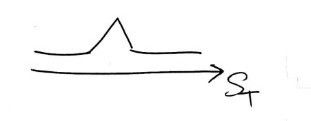
if my payoff looked like this it’d be amazing! Stable profits guaranteed, plus a little extra in a certain range. How great would that be!
But the person on the other side of that position —
would be holding a product with this profit structure. And like, would any investor on Earth sign up for that?? It absolutely would not sell.
For there to be liquidity in the product — i.e., for a real market of buyers and sellers to form — the form at the very top is the one that makes sense, right?
So the picture I drew earlier “as if it were obvious” — yeah, that’s actually the right picture. haha.
I went on a whole tangent about something pretty obvious.
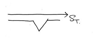
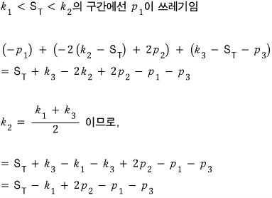
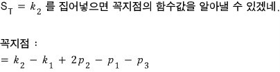
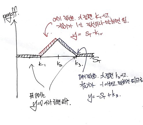
Anyway — while drawing the graph, I found the lower bound of the butterfly spread. Now let’s pin down that pointy part.
When the maturity price is in this range, of the call options:

are scrap paper. Garbage. The price is below their strike, so why on earth would you exercise the right to buy at a strike that’s higher than the market?
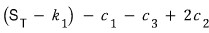
I wrote them in order — what comes from $c_1$, from $c_2$, from $c_3$.
Plug

into this and you get the y-coordinate of the peak. Right?
Peak:
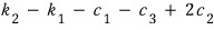
Now consider
In this range, only $c_3$ is scrap paper.
So:
I think that wraps up this part.
Butterfly can also be built from 3 put options. With the same condition:

For puts, higher strike → higher premium, so $p_1 < p_2 < p_3$.
Recipe:
- buy 1 of $p_1$
- sell 2 of $p_2$
- buy 1 of $p_3$
Draw each payoff against $S_T$ on one set of axes:
Yes yes yes easy~~
Sum them:
Yes yes yes easy.
The flat lower-bound part is already done, so let me characterize the jagged middle bits:
The above, actually… I went through it in a kind of long-winded way, but there’s a way to characterize the whole thing in one shot:
Pretend the premium is 0 and just draw it like this.
Once you do that, deriving the line equation in each piece is trivial, because you already know the x-intercepts.
Right?!?!?
And after you’ve characterized everything this way, just shift everyone equally
down by this much (parallel-shift in $-y$):
and now you have the function on every range, simply.
Oh — quick aside on butterfly spreads. The investor’s choice when using one is basically
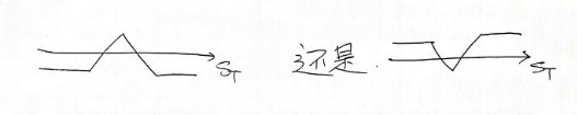
between these two, right?
So:
- the investor who picks the first is betting that future stock-price volatility will be small
- the investor who picks the second is betting that future volatility will be large
OK OK OK OK.
I can already hear the math majors loading their guns at me. Plausible~ plausible~
⑤ Calendar Spread
Calendar spread breaks just one of the rules from before — the same-maturity rule.
Up to now the options shared a maturity, “naturally.” Now we’re using options whose maturities are different (and instead, the strikes are the same!).
Hmm… so when you use 2 options — if the longer-maturity one is European, you’d have a problem at the short option’s expiry, because you can’t exercise European early. So:
- shorter maturity → American option
- longer maturity → European option
Let’s look at two combinations:
- short-maturity European call + long-maturity American call
- short-maturity European put + long-maturity American put
Spoiler: the payoff graph looks similar to a butterfly. Why it looks similar — let’s get there step by step.
First, the payoff of (short-maturity European call + long-maturity American call), evaluated at the European’s maturity!
So the American call’s payoff is drawn as a call value curve — time value included, present-value discounting included.
Looking at the two profit curves:
Yeah, like that, right!?!?
And if you very roughly sum them:
I was going on and on above about how it ends up like this. If someone asks why? — what do you say?
Time value. That’s the answer.
Time value is biggest at $S = k$, so the sum of the two is biggest there too.
(Another way to put it: the long call’s derivative is continuous everywhere, but the short call’s derivative is discontinuous at $S = k$. So the summed function’s derivative is also discontinuous at $S = k$. I think you can frame it that way too.)
Now — here’s an interesting question. What if we pick a $k$ that’s even more in-the-money (ITM)?
The call premium goes up, sure, but more importantly, the time value of the American call gets bigger. So when the peak point of the European-and-American sum sits at a more ITM $k$, the long call rises more.
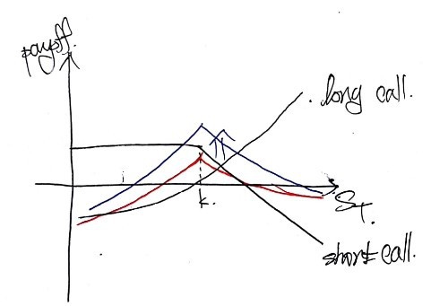
The peak goes up like this, and the range over which you turn a profit also widens. They say.
This is called a bullish calendar.
The reference I used: http://www.minyanville.com/trading-and-investing/how-to-trade/articles/SPY-time-time-value-price-options/7/31/2013/id/51068
The bearish calendar spread is the opposite, naturally. I’ll just say you can build the same kind of payoff using 2 short-maturity European puts and long-maturity American puts, slap a graph down, and breeze through.
And on that note I’m calling time on spreads.
This got way too long…. Cutting it here.
P.S.
Did you know? I converted all my blog posts to PDFs and I’m selling them :-)
https://blog.naver.com/gdpresent/222243102313

Blog post PDFs (ver. 2.0) for sale (the Physics and Finance I studied). Purchase info at the link~ Hi! If there are bits in the blog posts that feel unsatisfying, too… blog.naver.com
Originally written in Korean on my Naver blog (2016-12). Translated to English for gdpark.blog.