Binomial Option Pricing Model: Basics [Derivatives I Studied #15]

The stuff in Chapter 12 is actually material I already went through once before.

Rather than just dropping links, I’m going to copy-paste the whole thing over wholesale.

And then I’ll work some problems at the very bottom!

http://gdpresent.blog.me/220826670382

Financial Engineering Programming I Studied #4. Binomial Model — one period

OK so starting from Chapter 3, we’re doing the Binomial Model. Why “binomial”…

blog.naver.com

http://gdpresent.blog.me/220826694899

Financial Engineering Programming I Studied #5. Binomial Model — two period

Let’s keep going. We did one period, now it’s two period. heh. You know, that thing,,,,, that thing…

blog.naver.com

http://gdpresent.blog.me/220826741759

Financial Engineering Programming I Studied #6. Binomial Model — generalization (n period)

So far we’ve done one period and two period of the Binomial Model. Now we’re going to try…

blog.naver.com

Copy-paste begins

OK so starting from Chapter 3, this is the Binomial Model.

Why “binomial” —

Let me get into that first. Realistically, predicting stock prices is supposed to be flat-out impossible.

I mean — predicting a stock price… that just sounds like a totally absurd idea.

So apparently people thought:

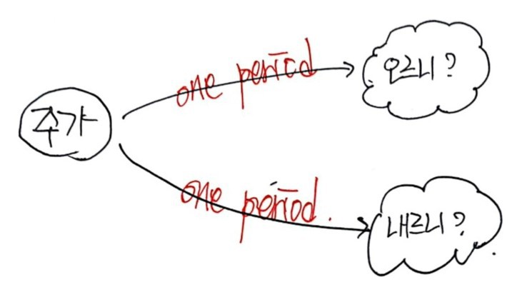
“OK fine, predicting stock prices precisely is impossible. But couldn’t we at least know whether the stock has gone up or down?!?!?!!!? If we could nail down even just that much, we could invest with some peace of mind!!!”

So the binomial model assumes that over some arbitrary period, a stock is either in a ‘risen state’ or a ‘fallen state’ — just those two states — and runs with that idea to find the theoretical price of an option…. That’s why it’s called ‘binomial,’ apparently.

More specifically:

“Only two probabilities exist for a stock price: the probability it goes up and the probability it goes down. (Like the discrete probability of a coin toss!)”

OK so first we’ll study just the ‘one period (1 cycle…(?))’.

That is, we look at just two time points: the present, and maturity. That’s it.

We’re going to compute the present value of a Call option for one period.

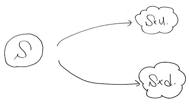
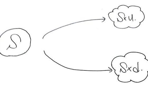
There’s an underlying asset whose current price is S, and let’s say after one period it’s either S×u (u > 1) or S×d (0 < d < 1).

And we’re going to build a risk-free portfolio. The portfolio: buy the underlying asset S, and short a call option!

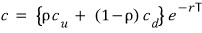
So the present value of the portfolio

$$P_{0}$$

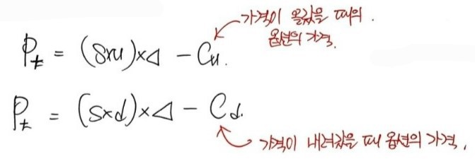
And the value of this portfolio one period later — heh —

<c_u, c_d — that thing from before: if S≥K then c=S-K, if S<K then c=0. That guy.>

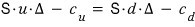
Since we built this as a risk-free portfolio, whether the price goes up or down, the value of the portfolio one period out has to be the same — so the following equation holds.

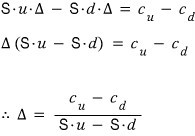
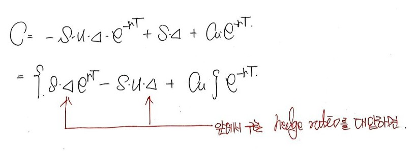
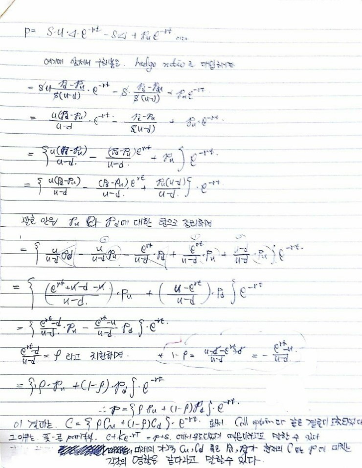
Now if we mess around with this a bit

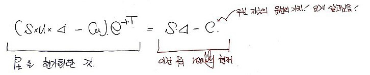
Δ stands for the number of shares we need to hold. This delta is called the ‘hedge ratio,’ apparently.

Also, the value of this portfolio has to equal the value before the one period too!!! Otherwise the words ‘risk-free’ would be empty.

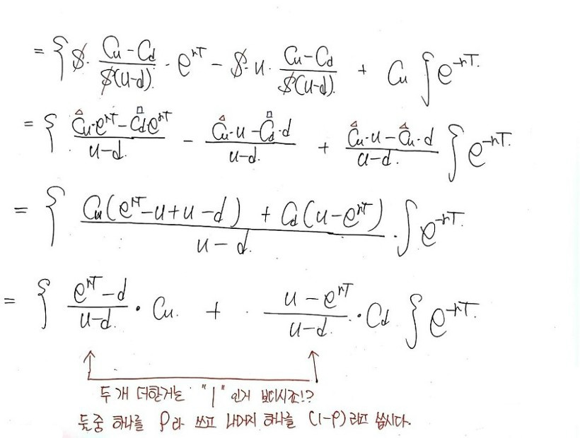
So now

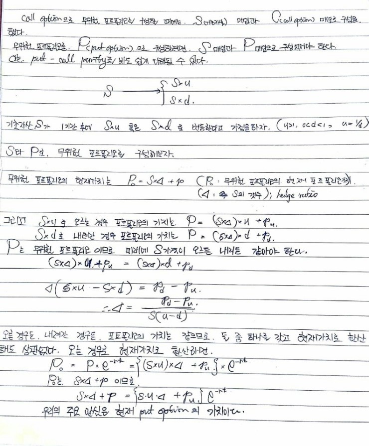
This blue guy!! is the value before we discount it back to present, and we can call this the ‘future expected value of c.’

One thing to notice: it’s in the form of a ‘weighted sum.’ This is going to be absolutely critical when we generalize later on!!! Weighted sum! heh

I’ll throw down some code for the above and then wrap up the post.

Sub Binomial_European_One_period() 'naming what I'm about to do, right here

Dim S as double, K as double, up as double, dn as double, rf as double, t as double, n as double

Dim rho as double, r as double, df as double, dt as double, c as double, cu as double, cd as double 'names of the things I'll use

S=100: K=100: up=1.1: dn = 1/up: rf = 0.05: t=1: n=1 'the relation up×dn = 1 is a financial engineering convention; more on this later

dt = t / n

r = exp(rf * dt)

df = 1/exp(rf * dt) 'apparently they make a discount factor like this because it's convenient when discounting to present, so they cook one up

rho = (r-dn)/(up-dn)

'these are my initial conditions~~

cu = Application.WorkSheetFunction.Max(S*up - K, 0)

cd = Application.WorkSheetFunction.Max(S*dn - K, 0)

c = ((rho)*cu + (1-rho)*cd)*df

End Sub

That red part — since I want to use Excel’s Max() inside VBA, I stuck Application.WorkSheetFunction. in front of Max(). Treating it as an application, just writing WorkSheetFunction. alone does the same thing, and dropping the WorkSheetFunction and writing only Application. also does the same thing — but this might differ a little by version,,,, so just take it as a reference. T_T

Anyway, the point is you cannot just write cu = Max(s*up - K, 0) on its own!!!! Why? Because Max() isn’t a function that lives inside VBA — it’s a function you have to drag in from elsewhere!!!!

lol lol lol

I priced the put option too, but suddenly I don’t feel like typing anymore,

and a few days ago someone showed me a ridiculously useful app…. So I’m planning to coast through the rest of my blogging life. lol lol lol lol

Let’s keep going. We did one period, now it’s two period. heh. You know that thing????? They say physics people only know three numbers. Is it the same for math people??? lol

The three numbers are 1, and 2, and then n. lol

I mean, financial engineering also looks like a field that got invented when mathematicians and physicists got hungry enough to jump into the financial markets…. lol

Yep. So we’ll derive two period and then immediately derive n period to do the generalization. And then we’re done, I guess. heh.

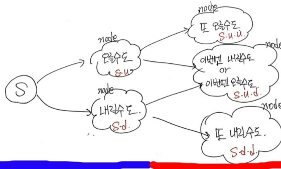
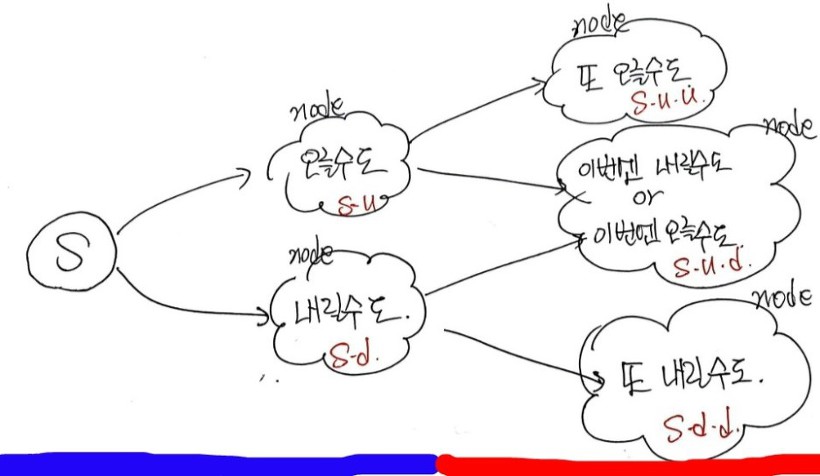
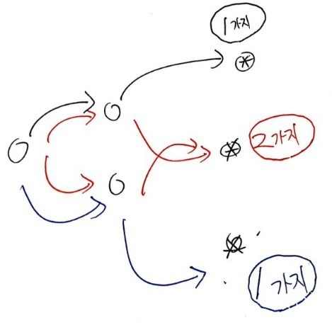
For two period, there are 3 possible cases at maturity, like this.

It’s easy!! heh. Since we’ve already done one period, this is a piece of cake.

The trick is just to look at it one period at a time. That’s why I deliberately drew a blue line and a red line at the bottom.

From the blue line’s perspective, this is just the one period we already handled, so the conclusion is the same as before.

What was it again?

Ah but — this is written entirely from the blue line’s perspective for the present Call value. Now there are 3 possible cases at maturity, so we need to shift our reference frame. (And we can’t forget — it’s European.)

So shift the reference to that red underline. And from the red underline’s perspective…… this is………..just………….

Same thing as looking at it like this, so the form has to be the same as above — only the subscripts change!!!!

OK OK… So in that case, we just swap the subscripts and write cu and cd.

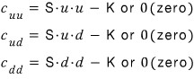
Now we need the values of c_uu, c_ud, and c_dd, but that’s also easy…!!! It’s just the call value at maturity —

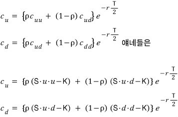
Done!!!

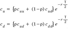
Now we need to express the present value of c in terms of c_uu, c_ud, c_dd!!!?!??

First

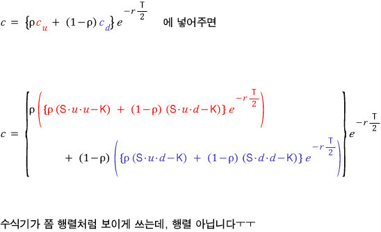
Make this substitution,

And now if we simplify!!!!!!!! Simplifying isn’t hard!!!

In one period, it was a weighted sum of 2 terms. In two period, it’s a weighted sum of 3 terms.

But now, if we read the formula a little,

First — the things in the blue boxes are the ‘values’ we’re adding up. (Of course, they’ve also been ‘discounted to the present’ by that exp factor in the back.) We add these three with weights —

Suu - K shows up with probability rho^2, Sud - K shows up with probability rho(1-rho), and Sdd - K shows up with probability (1-rho)^2.

And the black numbers? Those are ’the number of ways each thing can happen.’

Ohh I see — so for the possible values, probability × number of ways serves wholesale as the ‘weight,’ and the meaning of the binomial model is that it tries to price the current option price like this… T_T

(In the explanation above, I described it assuming cuu, cud, cdd definitely come out as suu-k and so on — but actually those values might not come out and could be zero!!!!! So strictly the description above is wrong. But I figured explaining with concrete numbers makes it more tangible, so I just developed the formula as ’numbers.’)

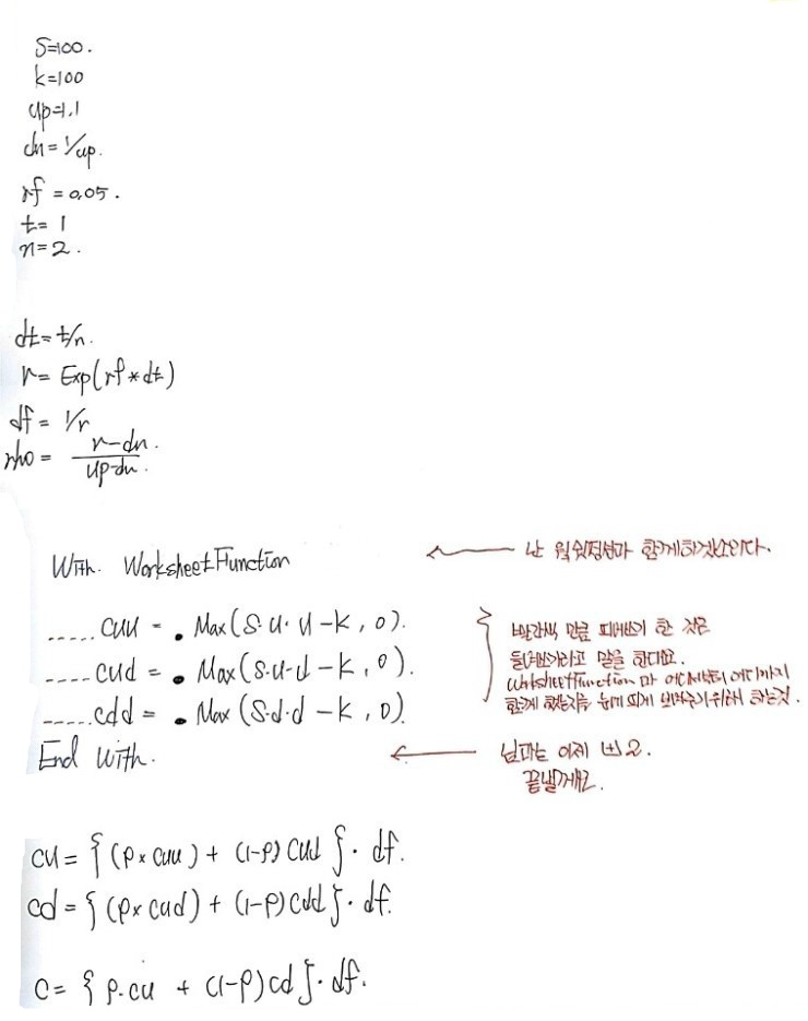
OK so two period is done, now we head toward n period, but I’ll code this one up real quick first and move on. The thing we’re picking up here is the use of With ~ End?????

Other than that there’s nothing, so I’ll just

So far we’ve done one period and two period of the Binomial Model. Now we’re going to try n period.

That is — generalization.

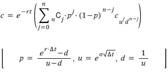
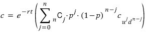
First, I’ll just throw the generalized formula out. Then I’ll dissect it bit by bit and interpret it, so do not be shocked by the formula I’m about to throw down right now!!!!!!

※Warning: heart-stopper※

Eek!!!!!!!! My heart stopped… T_T Ahh…..

To look at this formula again, let’s revisit the two period formula.

Aha… So why is that sigma (Σ) in the generalized formula?!?! Looks like it’s just there to express the weighted sum compactly.

Now let’s look at the new characters that showed up and then move on.

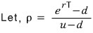
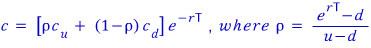
First: what is p?!?!?!?!? Wasn’t that spot originally for ρ(rho)?!?!?!

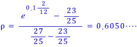
- Originally rho was

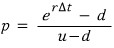
which we got via substitution, and the meaning was: if the probability of price rising over period T was ρ, then (1-ρ) was the probability of falling — that’s basically it. But now we can’t say T anymore. Instead of saying “over T,” we have to say “over a unit of time.” Because we’re slicing the whole T into finer and finer pieces and asking: during that one slice of time, did the price go up or down —

OK, p is settled. It’s just being used in place of rho… heh

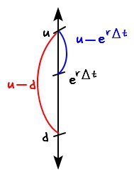
(But let me briefly mention why this can be read as a ‘probability.’ You can think of it as something like ‘geometric probability.’ For now, exp(rΔt) is the rate at which value grows on its own (call it a multiplier). u is the up-multiplier, d is the down-multiplier. So u-d is the overall ‘size,’ and exp(rΔt)-d is the size in the upward direction within that u-d range, so to speak. I’ll throw a picture below for this. heh)

Second: what’s u all of a sudden?????

excuse me?!?!?!?!

Why exactly the growth rate u is defined in that form with σ and a time variable — where that comes from, I can’t actually answer right now, apparently… T_T Sorry. My math is lacking. T_T (Also, the volatility itself isn’t a constant — it’s tangled up in a complicated way with other variables… Strictly speaking that’s the case, but since I can’t get into that right now either, for the time being we’ll treat it as a constant and solve problems.)

Third: u = 1/d

The basis for this lies in the Cox-Ross-Rubinstein model, apparently… heh. Let’s punt on examining the CRR model until next time.^^heh

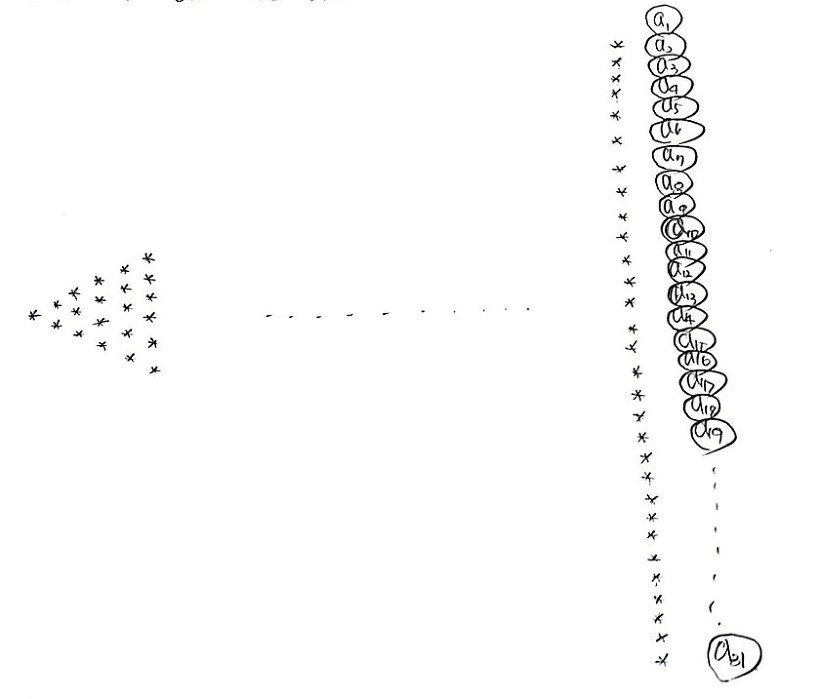
Now about that weighted sum — even though it’s in a form anyone can grasp easily, let me ramble about it once and then move on.

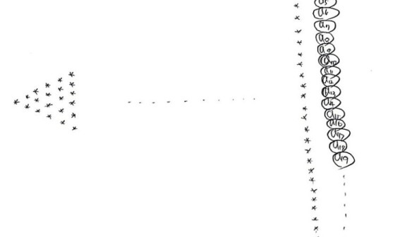
For example, say there are 31 possible option prices at exactly time T at maturity. We need to take the weighted sum over all 31. That’s the sigma.

OK then — what probability does the value

representing a_1 show up with? It must have gone up all 30 times, so it’s p^30. (one period: 2 cases, two period: 3 cases — so 31 cases means it’s currently 30 periods.)

And the number of ways it can happen is 1. But rather than just saying “1 case,” for purposes of understanding the weighted sum, it’s better to say it’s

cases.

What about a_2???? a_2 means: out of the 30 price-movement opportunities, only 1 went down, and the other 29 went up.

So the probability that a_2 shows up is (p^29)*(1-p). And the number of ways it can happen — since out of 30 chances we just need to pick which 1 was the down move —

cases, you could say.

Just one more last one! a_17! Let’s just do this one. Random number. a_17 is the option value where 16 out of 30 movement opportunities went down and 14 went up, so the probability of becoming a_17 is (p^14)((1-p)^16), and the number of ways that can happen is

aha

So that weighted sum somehow… makes sense now, why it ends up as that kind of sum!!! heh

- What goes into the weighted sum is

which is the price of the call option. But I didn’t say this explicitly above because the call price might be some number, but might also be zero (nonlinear), so I just called it the call price!!! So some of those could be zero. heh

P.S.

Did you know? I converted all my blog posts to PDF and I’m selling the PDF materials. :-)

https://blog.naver.com/gdpresent/222243102313

Blog post PDF (ver.2.0) for sale (Physics and Finance I Studied)

Purchase info below. ~ Hello! If there are parts of the blog posts you find unsatisfying, too much…

blog.naver.com

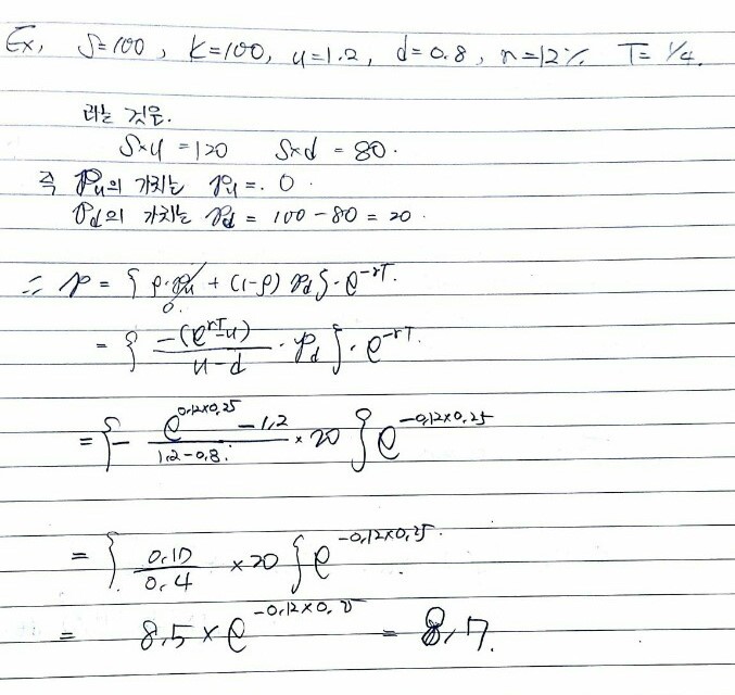
Prob 12. 9

The current stock price is 50.

Suppose 2 months from now the stock price is either 53 or 48.

The risk-free rate is 10% (continuously compounded).

What’s the price of a European call with maturity 2 months and K=49?

We already derived everything, right???? Just use it;;;;.

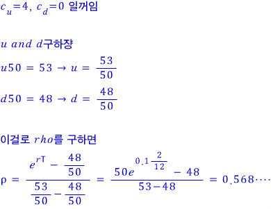
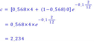
Ingredients ready!!!

Prob 12. 10

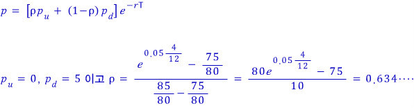
The current stock price is 80. Suppose 4 months from now it becomes either 75 or 85.

The risk-free rate is 5%. Find the price of a European put with maturity 4 months and strike 80!

Ingredients ready!

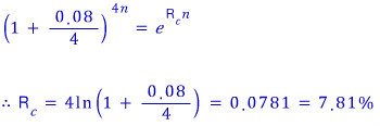
Prob 12. 11

The current stock price is 40. Suppose 3 months from now it becomes either 45 or 35.

The risk-free rate is 8% quarterly compounded.

What’s the price of a European put with maturity 3 months and strike 40?

First off, that quarterly compounding is ridiculously annoying.

Now, well, I can solve this in my sleep.

Ingredients ready?

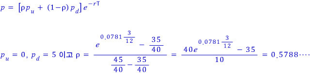
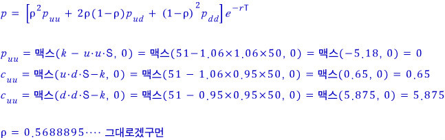
Prob 12.12

The current stock price is 50.

Every 3 months the stock price either rises 6% or falls 5%.

The risk-free rate is 5% continuously compounded.

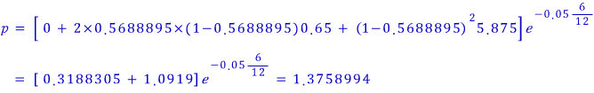
What’s the price of a European call with maturity 6 months and strike 51?

Oh ho!!! This one’s a two period problem?

But at this level we can crunch it by hand.

Ingredients ready.

Prob 12. 13

From problem 12.12 above, compute the European put price with the same maturity (6 months) and strike 51, and show that put-call parity holds.

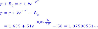
If we take c=1.635 and run it through put-call parity once —

Wow, incredible, absolutely incredible;;;;.

Prob 12. 14

The current stock price is 25. Suppose 2 months from now it’s either 23 or 27.

The risk-free rate is (continuously compounded) 10%.

Suppose the stock price at maturity is

What’s the price of a derivative whose payoff 2 months later is

This one we have to solve using the fundamental principle behind every option price we’ve been computing so far.

The fundamental principle was actually ’expected value.’

That was the fundamental principle.

Lucky for us — there are only 2 situations at redemption.

The case where the payoff is 27 squared, and the case where the payoff is 23 squared.

The probability of each is

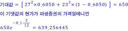
So the expected value of the derivative is

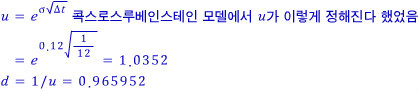
Prob 12. 15

When you build a binomial process to value an option on a foreign currency, compute u, d, and p.

One period is 1 month, domestic rate is 5%, foreign rate is 8%, volatility is 12%.

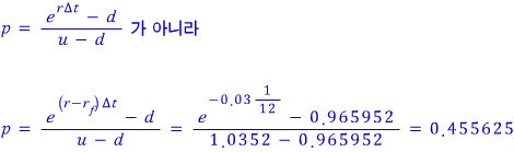
Huh?? That’s it?

Originally written in Korean on my Naver blog (2016-12). Translated to English for gdpark.blog.