Deriving the Black-Scholes Formula from the Binomial Model

So this chapter is about the option pricing formula that pops out of the Black-Scholes model, you know??

That~~~ thing called the BS formula that we kinda half-baked our way through in financial engineering class??

The whole point is gonna be: get a feel for what’s going on, and use that formula to think about it.

But before we just go around plugging numbers into the BS formula —

I think we should at least derive the thing once. You know, sanity check. Make sure it’s actually okay to use.

OK so this BS “pricing formula” — you can summon it into existence with a handful of assumptions.

B and S… Black and Scholes assumed stock returns follow a log-normal distribution, that returns are independent across time, that volatility is constant… oh and the interest rate is constant too…

Plug all that in, crunch through it, and the formula falls out.

Once it falls out, though… it’s wayyyy too hard.

Can’t we get there in some easier way???????

That, my friends, is exactly what the binomial model is for.

You can derive the BS formula straight out of the binomial model!!!

So my plan: take the binomial model, send $n \to \infty$,

watch the BS formula plop out,

and then we get to happily use it for the rest of the chapter.

Translation: this is not gonna be a super rigorous post…..(sigh) huhuhuhuhuh

In some future post I’ll go through deriving BS the proper way — from the assumptions —

and also the path through the Black-Scholes PDE to the BS formula,

and stuff like that — once I’m done with all the postings before that one,

I promise I’ll get to it!~

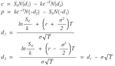
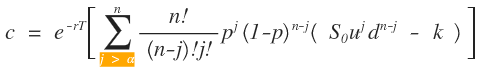
Alright, let’s drag the BS formula out of the binomial model.

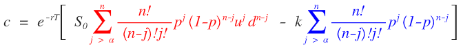
In the previous post,

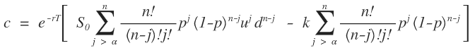
we saw that the option price in the binomial model is

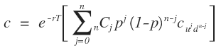
this thing.

I’m gonna rewrite it slightly.

Same thing, just dressed up differently:

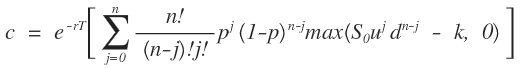
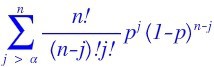
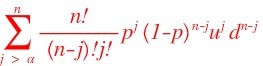
OK so — among the terms inside that big sigma ($\Sigma$),

a bunch of them are gonna be zero anyway.

So I wanna kick those out…. heh

Here’s how to kick them out:

these are the only ones I want to keep — toss the rest —

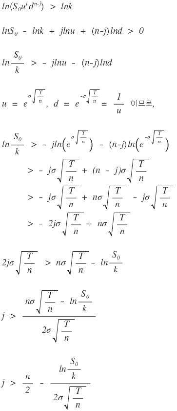
so in the sigma above,

if I just slap a $j$ condition on it like this, boom — the sum only includes the nonzero terms.

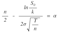
That weird-looking number on the right? I’m gonna call it $\alpha$.

Then the sigma can also be written like this:

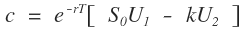
And I’m gonna split it into two pieces:

That’s fine, right?????????

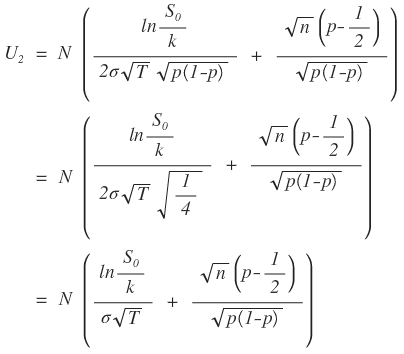
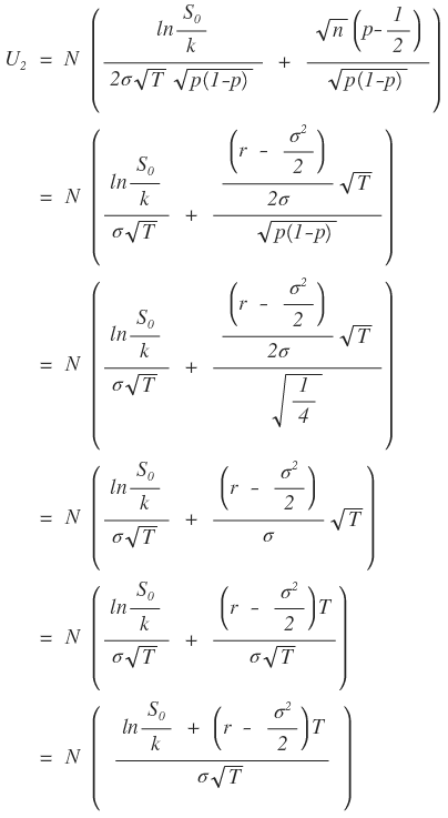
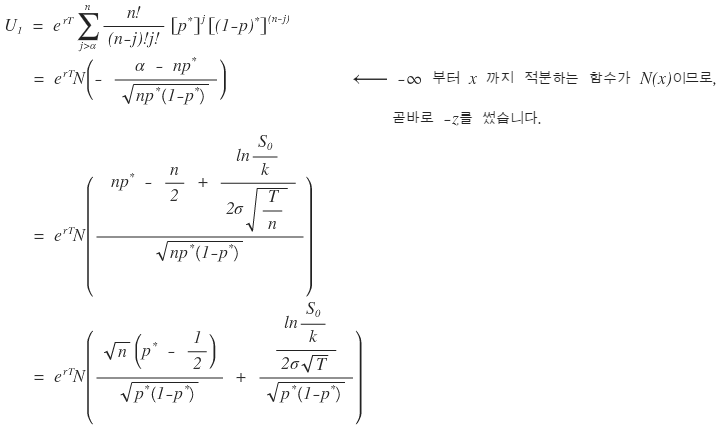
The red term I’ll call $U_1$,

and the blue one $U_2$.

Okaaaaaaaaaaaay. Let’s stare at $U_2$ first.

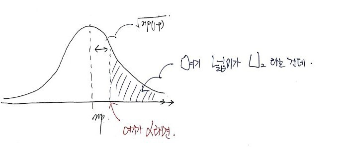
We know that the binomial distribution, when you crank $n$ to infinity, becomes the normal distribution.

Mean is $np$, variance is $np(1-p)$.

This is a thing they literally prove in high school,

and if you look at $U_2$, it’s saying: sum up all the probabilities for the cases where the number of up-moves $j$ is bigger than $\alpha$.

So (pretending $n$ is already huge) starting from $N(np, np(1-p))$,

we just whoooosh sweep up all the probability mass to the right of $\alpha$, right?

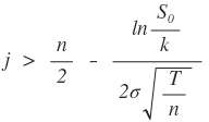
How do you actually compute the cumulative probability up to $\alpha$???

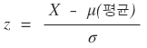
Easy — standardize it.

In the normal distribution, the position of $X = \alpha$,

translated into the standard normal distribution, sits at:

so $\alpha$ lands at:

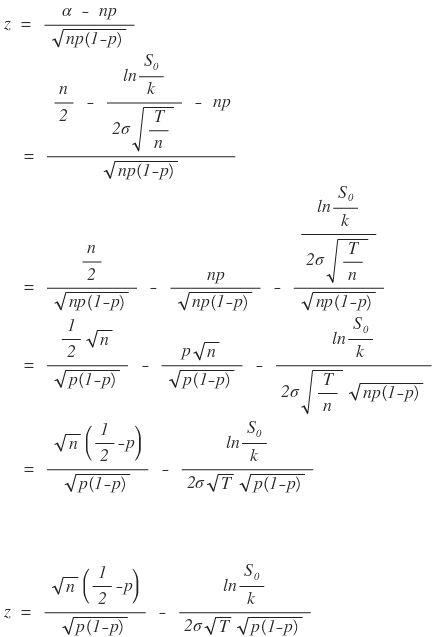
That’s where $\alpha$ lives in the standard normal.

And remember, what we actually want is $U_2$:

This is a sum over the binomial,

but the sum doesn’t go from $0$ to $n$ — it only covers the part above $\alpha$.

So what $U_2$ really represents is

this area right here.

And since a Gaussian with mean $np$ and that variance is kinda annoying to work with directly,

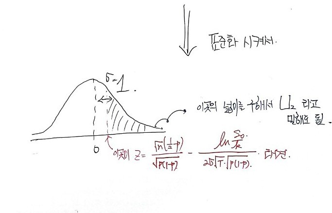
I’m gonna standardize it like this and then talk about the area.

Still not satisfied though.

Let me massage it one more time:

ok ok ok ok ok.

So:

the area from $-\infty$ up to that number above, in the standard normal, is $U_2$.

Which means, as of right now,

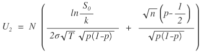
we can say this much.

Now about those $p$’s:

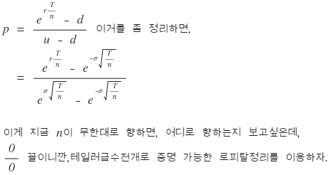
so in the end,

up to here we’ve nailed down.

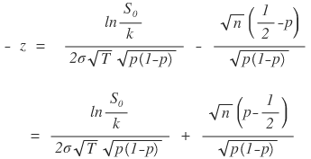
“Why didn’t you touch the back term??” — glad you asked.

That term has $n \to \infty$ multiplying $(p - 1/2) \to 0$. That’s $\infty \times 0$.

Indeterminate. Gotta look at it more carefully.

This part actually wrecked me,

and right when I was about to give up, I stumbled into it by sheer luck.

So the math is a little… let’s say, not pretty…..

Bear with me.

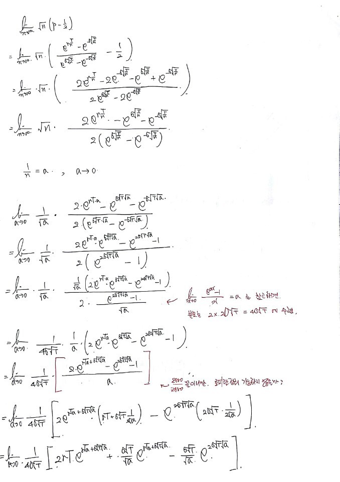
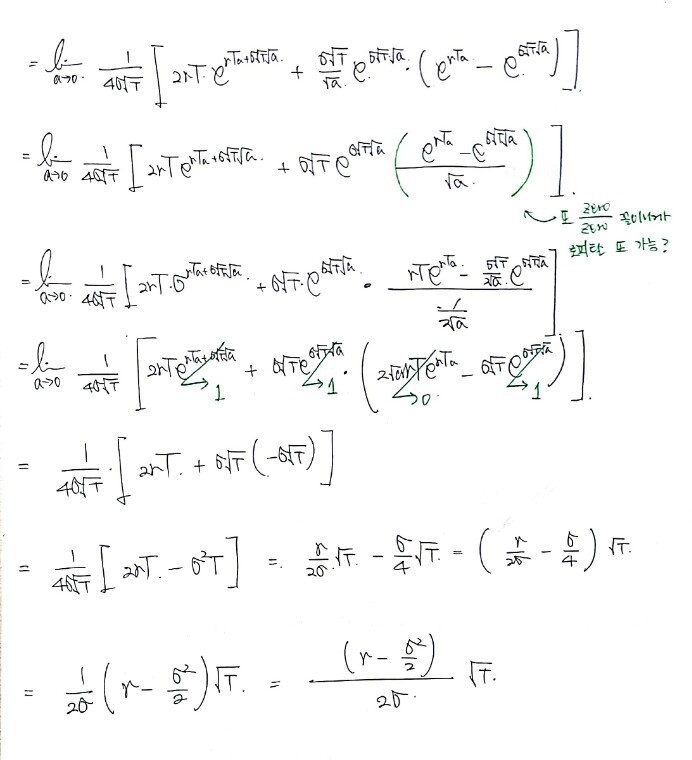
Barely.

Pulled it off by the skin of my teeth.

$N(d_2)$ does come out, doesn’t it?? (sob)(sob)(sob)

Now I gotta show that $U_1$ gives us $N(d_1)$,

ugh… haha when am I gonna finish this lol lol lol lol lol lol lol lol lol lol lol lol lol lol

lol lol lol lol lol lol lol lol lol lol lol lol lol lol lol lol lol lol lol lol lol lol lol lol lol lol lol lol

This was $U_1$,

and I want to recycle the $U_2$ trick as much as possible, so

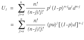
I wrote it like this.

And looking at it again —

$pu$ is basically the “expected up-rate (?)” and $(1-p)d$ is the “expected down-rate (?)”, right?

So I’m gonna rewrite it once more:

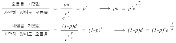
Plug it in:

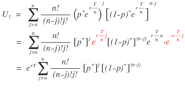
The red thing yeets itself, $\exp(rT)$ falls out,

and the sigma now has the exact same structure as when we handled $U_2$!!!!!!!!!!!!!!!!!!

Yesss~~~~

So by the same logic,

we just need to figure out where $p^*$ goes as $n \to \infty$,

and where $\sqrt{n}(p^* - 1/2)$ heads.

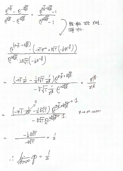
$\lim p^*$ is easy.

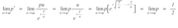
Now… $\sqrt{n}(p^* - 1/2)$……….

This one really had me in tears… I’m bad at math,

and I have a sneaking suspicion I’m taking the long way around to a place I could’ve reached in one move….

Sorry (sob)(sob)(sob)(sob) heh heh heh

But we gotta get to the destination, so… (sob)(sob)

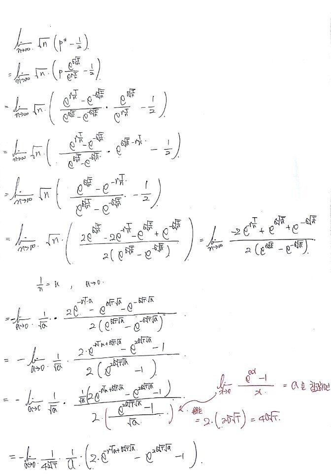
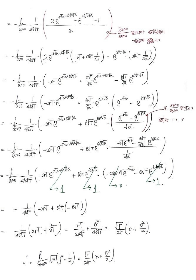
In the end;;;

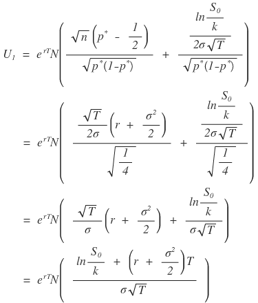
Oh wow…. finally.

$U_1$ and $U_2$ — DONE!!!!!!!!!!!!!!!!!!!!!!!!!!!!!!

Which gives us

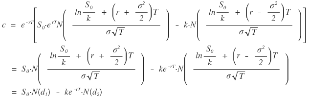
There it is…………

(shaking)(shaking)(shaking)(shaking)(shaking)(shaking)

I really should not have started this lol lol lol lol lol

lol lol lol lol lol lol lol lol lol lol lol lol lol lol

How long did this take me to write lmao

There are 100% gonna be typos…….

Oh!!!!!!!!!!!!!!!!!!!

What about the put option,

you want me to derive that one with the binomial model too?????

Sorry. Not happening.

We’re taking the easy way out — Put-Call Parity…….

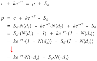
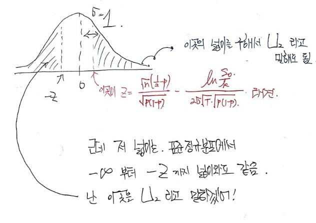
The step with the red arrow

is just a property of the Gaussian.

Like I said above: (integral from $x$ to $\infty$)

$=$ (integral from $-\infty$ to $\infty$) $-$ (integral from $-\infty$ to $x$)

$= 1 -$ (integral from $-\infty$ to $x$)

$=$ (integral from $-\infty$ to $-x$)

That move!

One more quick thing before I wrap up.

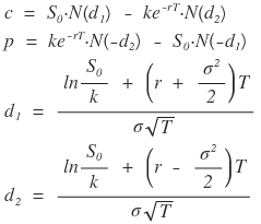
We derived this — but does this formula even make sense???????

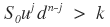
Imagine the current stock price $S_0$ is, like, monstrously, absurdly, super-mega-ton huge.

Then for a call option, the probability of exercising it down the line is basically 100%, right???????????

If $S_0 \to \infty$, then $d_1$ and $d_2$ also go to infinity, right?

Then $N(d_1), N(d_2) \to 1$.

So the price of the call

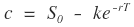
converges to this —

but wait, what does that even mean….. the right-hand side is literally the value of a forward contract, isn’t it?

Why???????????????

Because the stock price is so absurdly high that exercising at strike $k$ is a done deal,

it collapses to the price of a forward — which is the totally-certain version of the same trade!!!

On the flip side, the value of a put

has $N(-d_1), N(-d_2) \to 0$,

and the put price goes to 0…

Because the probability of it ever being exercised is ~zero….. value goes to zero….

Oh ho?!?!?!! This formula!! actually makes sense?!?!?!!!!

OK this got way too long.

I’ll grind through some practice problems before moving on —

hmm… I’ll do them in the next post.

Originally written in Korean on my Naver blog (2016-12). Translated to English for gdpark.blog.