Gauss's Law: Electric Flux and Gaussian Surfaces

Editorial correction — 2026-09-08

This English edition keeps the informal voice and illustrations of the original Korean study notes from 2014. It corrects the explanations of signed flux, unit normals versus area vectors, and zero net flux versus local charge density. Two small fragments labeled as “unit area” and the volume-integral derivation have been replaced by the explicitly corrected mathematical text below. All original source images are preserved. The sphere calculation with the red area integral already has the correct powers, constants, and result; its notation is clarified here.

Did we learn Gauss’s law in high school? I honestly can’t remember. Haha.

Maybe you’ve landed here after wondering what Gauss’s law actually means. Let’s start with a ridiculous picture, then work our way toward the mathematics.

A wildly impractical soy-sauce experiment

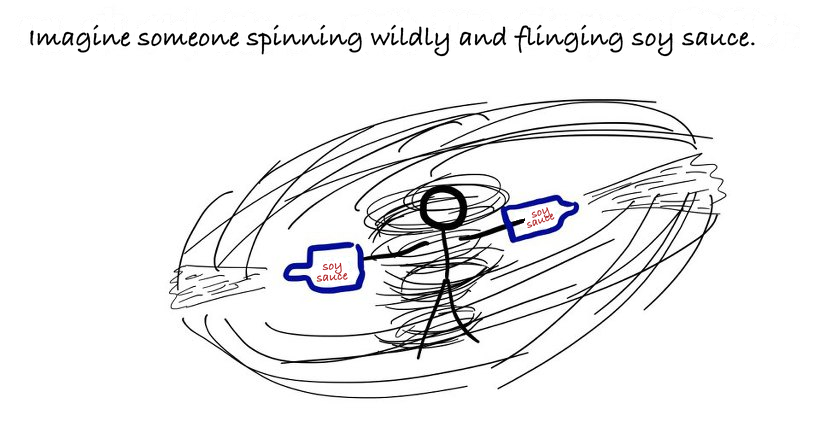
Imagine someone spinning wildly and flinging soy sauce in every direction. For this story, suppose the droplets keep traveling straight outward forever. Yes, we’re making some heroic assumptions!

Now imagine a tightly packed crowd surrounding this person at a radius of 5 m. Everyone gets soy sauce on their clothes. Move the entire crowd out to 50 m: the sauce still reaches them. What about 100 m? Or 1,000 m? Or 103,420 m? How about 1,394,830,980,340 m? Apparently I don’t know when to stop.

Compare these as separate arrangements, with the same amount of sauce emitted each time. If the crowd completely intercepts it, the total amount caught stays the same, even though it is spread over a larger enclosing surface farther away. That is the intuition I want to borrow.

There are limits to this picture. A ring of people on the ground is not a closed surface in three dimensions; imagine a complete enclosing shell instead. Real droplets carry material, while electric field lines are a drawing convention. And a Gaussian surface is imaginary: it neither catches nor blocks the electric field. Keeping the total flux fixed does not keep the local field strength fixed.

So the soy sauce gives us a starting point, not a complete proof. Let’s put the bottles down before this gets any messier.

What electric flux measures

The electric field is a vector. At any point, an arrow can show its direction, and the arrow’s length can represent its magnitude. Drawing an arrow at every point in space would be quite a job, though. Field lines give us another useful picture.

A field line’s tangent follows the field direction. Within a fixed drawing convention, more lines passing through a small area perpendicular to the field represent a stronger field. This is an area density, not a count per unit volume. The finite number of lines in a sketch is our choice; nature does not supply a fixed number of drawn arrows. See the University of Texas at Austin’s explanation of electric field lines.

To define flux, choose an orientation for a surface $S$. Let $dA$ be a small positive area and let $\hat{\mathbf n}$ be its unit normal. The electric flux is

$$ \Phi_E(S)=\int_S\mathbf E\cdot\hat{\mathbf n}\,dA. $$

This is a signed scalar. Each patch contributes the field’s normal component multiplied by its area. We add those scalar contributions; we do not add the field vectors themselves. Flux has SI units of $\mathrm{N\,m^2/C}$.

For a closed surface, we choose the outward normal and put a circle on the integral sign. This original formula uses $\Phi_S$ for that closed-surface flux:

An outward-pointing field gives a positive contribution, an inward-pointing field gives a negative contribution, and a field tangent to a patch gives zero. The ordinary surface integral above also applies to an open surface once its orientation is chosen.

Here is the local patch picture:

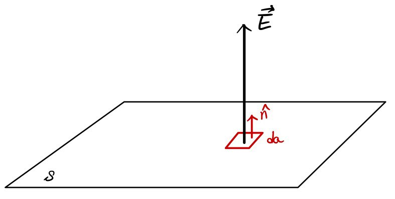
The drawing labels the scalar patch area $da$; we’ll write it as $dA$ to keep it distinct from the area vector. This flat patch illustrates the orientation at one place. It is not, by itself, a closed Gaussian surface. The field happens to be parallel to the normal in this sketch; in general, the dot product selects just the normal component.

A point charge at the center of a sphere

Now put a positive point charge $q$ at the center of a sphere of radius $a>0$, with no other charges or imposed field contributing to this example. The outward arrows in the sketch match that positive charge:

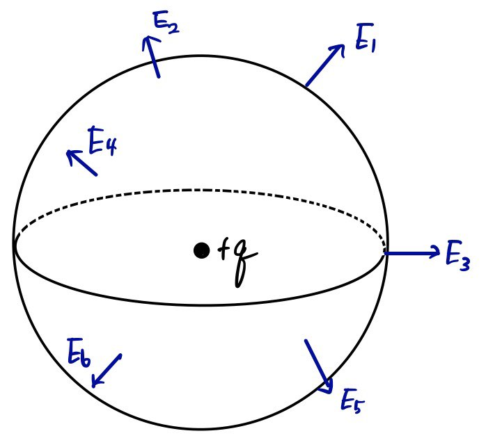
The sphere is our imaginary enclosing surface. To calculate flux, we need the area vector at each small patch. Here is the corrected notation replacing the original “unit-area” fragment:

$$ d\mathbf a=\hat{\mathbf n}\,dA. $$

We take $\mathbf E\cdot d\mathbf a$ on each patch and integrate over the sphere. The field vectors at different patches have different directions. The original notes label some of them

and, continuing the sequence,

Their magnitudes are equal because every patch is the same distance from the sole source charge. The six arrows in the sphere drawing are schematic samples, not six separate physical field lines that we must count.

One more notation point is worth slowing down for. In place of the second original “unit-area” fragment, we distinguish

$$ \lVert\hat{\mathbf n}\rVert=1, \qquad \lVert d\mathbf a\rVert=dA. $$

The unit normal is dimensionless. The area element $dA$ and area vector $d\mathbf a$ have units of square metres; neither has a fixed magnitude of one. The hat belongs to the direction vector. “But GD park, weren’t you trying to keep this light?” I am! Keeping two different things from sharing one confusing name actually makes the calculation easier.

We now evaluate the closed-surface flux:

For this centered sphere, the outward normal is the radial unit vector $\hat{\mathbf r}$. Thus

$$ \mathbf E(a)=\frac{q}{4\pi\epsilon_0a^2}\hat{\mathbf r}, $$$$ d\mathbf a=\hat{\mathbf r}\,dA. $$

Since $\hat{\mathbf r}\cdot\hat{\mathbf r}=1$, the dot product becomes the constant outward normal component of the field times $dA$. Here is the angular-integration route from the original notes:

To spell out its limits, the polar angle satisfies $0\leq\theta\leq\pi$ and the azimuthal angle satisfies $0\leq\phi\leq2\pi$. The scalar area element is

$$ dA=a^2\sin\theta\,d\theta\,d\phi, $$

so

$$ \Phi_E=\frac{q}{4\pi\epsilon_0} \int_0^{2\pi}\int_0^\pi\sin\theta\,d\theta\,d\phi. $$

The angular integral is $4\pi$, giving $\Phi_E=q/\epsilon_0$.

Or we can use the sphere’s area directly. This is the same calculation, so feel free to take whichever route clicks first:

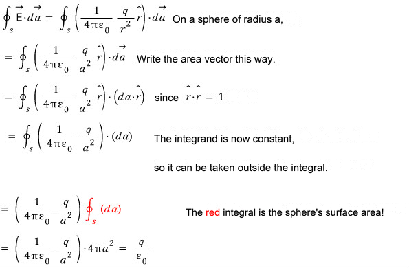
In this image, the scalar $da$ inside parentheses means our $dA$, and multiplying it by $\hat{\mathbf r}$ forms the area vector. The red integral is the sphere’s total surface area, $\oint_S dA=4\pi a^2$. The coefficient is constant over the centered sphere, so

$$ \Phi_E=\frac{q}{4\pi\epsilon_0a^2}(4\pi a^2) =\frac{q}{\epsilon_0}. $$

There it is! Increasing the radius weakens the field as $1/a^2$, while the area grows as $a^2$. The net flux stays the same.

We assumed $q>0$ to match the outward arrows. If $q<0$, the field points inward and the signed normal component and flux are negative; the result $q/\epsilon_0$ still holds. If the charge is off-center but remains inside the sphere, the net flux is still $q/\epsilon_0$, although the field is no longer uniform in magnitude or normal to every patch. We cannot use “one constant field value times the area” in that case.

Who chooses the Gaussian surface?

Wait a second—what exactly is a Gaussian surface? Who chose that sphere?

We did! A Gaussian surface is an imaginary closed surface chosen for a calculation. It can have any suitable shape or size. A sphere was convenient here because the centered charge made the field simple on it. In another problem, a cylinder or a box might be more useful. Choose a boundary that does not pass through an ideal point charge.

Gauss’s law always relates net flux to enclosed charge. With enough symmetry, it can also help us find the field’s magnitude and direction. Without that symmetry, knowing one total flux usually does not tell us the field at each point; another method may be easier. Many introductory exercises deliberately use symmetric charge distributions so that we can practice this choice.

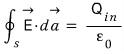
Now let there be several charges inside. We’ll write their signed net charge as $Q_{\mathrm{in}}$. The integral form of Gauss’s law is

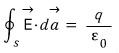
For comparison, our single enclosed point charge gave

With several point charges, add their signed charges, including only those inside the volume $V$:

$$ Q_{\mathrm{in}}=\sum_{\mathbf r_i\in V}q_i. $$

Positive and negative charges can cancel in this sum. The law then reads

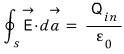
Whatever the field does from patch to patch, the sum of its signed flux contributions is

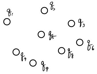
Here is the charge distribution from the original sketch:

And here are three possible enclosing surfaces:

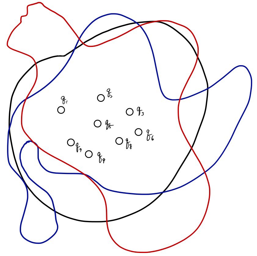
Think of those contours as sketches of closed surfaces in three dimensions. Each encloses the same depicted charges, so each has the same net outward flux. The shape can change the field’s angle and strength at individual patches, but it does not change the enclosed signed charge.

We might not know the contribution at a particular patch,

yet the total over the closed surface,

must equal

The field in that integral is the total electric field. Charges outside the surface can change it at each patch, but their contributions to the net flux through the closed surface cancel. Only enclosed charge appears on the right-hand side. The constant $\epsilon_0$ remains the permittivity of vacuum; the charge here is total charge, not just a selected subset of free charges.

From an enclosing region to a local equation

The divergence theorem lets us express the same flux using quantities inside the volume. These steps are the corrected mathematical replacement for the original volume-integral image. We use a closed-surface integral over the boundary and ordinary volume integrals over the interior.

Let $S=\partial V$ be the outward-oriented boundary of a volume $V$. Write $\rho(\mathbf r)$ for the total charge density, measured in $\mathrm{C/m^3}$. For a continuous distribution,

$$ Q_{\mathrm{in}}=\int_V\rho(\mathbf r)\,dV. $$

Gauss’s law gives

$$ \oint_{\partial V}\mathbf E\cdot d\mathbf a =\frac{1}{\epsilon_0}\int_V\rho\,dV. $$

For sufficiently regular fields and a suitable boundary, the divergence theorem gives

$$ \oint_{\partial V}\mathbf E\cdot d\mathbf a =\int_V\nabla\cdot\mathbf E\,dV. $$

Combining them,

$$ \int_V\left(\nabla\cdot\mathbf E- \frac{\rho}{\epsilon_0}\right)dV=0. $$

The crucial point is that this identity holds for every admissible volume $V$, not merely one surface we happened to choose. Where the field and density are regular, it implies the local equation

$$ \nabla\cdot\mathbf E=\frac{\rho}{\epsilon_0}. $$

That is the conclusion shown in the original notes:

This is the differential form of Gauss’s law, one of Maxwell’s equations. The integral form describes a whole enclosing region; the differential form describes the local source of the field. Neither viewpoint requires a giant sphere.

Ideal point charges need one extra qualification. Their fields are singular at the charge positions, so the ordinary pointwise derivative is not defined there. The same law holds in the distributional sense, with delta functions representing point sources. Away from those sources, the ordinary local equation applies. The University of Texas at Austin’s treatment of Gauss’s law develops this distinction in detail.

We will use this move between surface and volume integrals again. It can look like a lot of manipulation the first time, but it gives us a useful change of viewpoint.

A reader’s question: how can both fluxes be zero?

A question prompted this addendum. These two situations are clearly different:

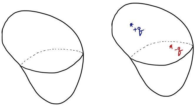
On the left, the enclosed charge,

is zero because there are no charges inside. On the right, the enclosed charge,

is also zero, because the two signed charges add to $q+(-q)=0$. Therefore, the net flux through each enclosing surface is zero.

That does not make the two electric fields the same. If we additionally assume that there are no external charges or imposed fields in the left example, the field is zero and every patch contributes zero flux. If an external field is present, an empty region can instead have a nonzero field whose inward and outward fluxes cancel. No enclosed charge, by itself, does not mean no field.

On the right, the separated charges generally produce a nonzero field. The signed scalar contributions $\mathbf E\cdot d\mathbf a$ cancel when integrated over a surface enclosing both charges:

$$ \oint_S\mathbf E\cdot d\mathbf a =\frac{q-q}{\epsilon_0}=0. $$

So my informal “something plus something else equals zero” refers to signed flux contributions, not a sum of electric-field vectors. Nor does this one zero integral say that the local divergence is zero everywhere. The divergence vanishes at charge-free points, while the ideal charges themselves contribute positive and negative point sources. A smaller surface enclosing only one of them has flux $+q/\epsilon_0$ or $-q/\epsilon_0$.

If this is your first encounter with electromagnetism, I wouldn’t expect everything to click in one reading. Speaking as a very ordinary learner myself, it certainly helps to work through problems. Eventually you’ll find yourself thinking, “Ah, choosing the surface this way makes the field calculation much easier!”

Keep practicing, and study well.