Electric Potential and Voltage

This time, let’s look at electric potential. When I hear the term, I immediately think of voltage, and then the number 220 V pops into my head. But what does potential actually mean?

Editorial correction, 2026-09-09: This English edition of my original study note clarifies the distinction between potential and energy. The first, second, third, fourth, and sixth equation images have been replaced by typeset expressions. The first, second, third, and sixth needed corrections to missing differentials, vector dot products, or the first minus sign in the point-charge calculation. The fourth image contained the correct recap equations, but its vector arrows were clipped. The original image files are preserved.

Conservative fields and scalar potential

We are working in electrostatics: the charges producing the field stay fixed. The electric field has zero curl,

$$ \nabla\times\mathbf E=\mathbf 0. $$

To use zero curl as a test for path independence, suppose the field is continuously differentiable on a simply connected open region. That means, roughly, a region where every closed loop can shrink to a point without leaving it. Under these conditions, the line integral between two points depends only on the endpoints. Zero curl alone is not a global guarantee on every region, and this argument does not cover arbitrary time-dependent electric fields. Our paths also avoid field singularities.

A force whose work is independent of the path is called conservative. The electrostatic force is conservative, so we can describe it using a scalar potential. After choosing a reference, the electric potential assigns a single number to each position.

I had heard this explanation plenty of times before it really sank in. The equation makes the idea much more concrete. Let the scalar function $V$ be continuously differentiable, and let $C$ be a piecewise smooth path from $\mathbf a$ to $\mathbf b$ within that region. The gradient theorem says

$$ \begin{aligned} &\int_C \nabla V\cdot d\mathbf r\\ &=V(\mathbf b)-V(\mathbf a). \end{aligned} $$

The dot product pairs the gradient with the tiny vector displacement along the path. Integrating these changes gives the difference between the endpoint values.

This is the same idea as the familiar one-dimensional fundamental theorem of calculus. For a continuously differentiable function $f$,

$$ \int_a^b \frac{df}{dx}\,dx=f(b)-f(a). $$

In both cases, adding up the small changes recovers the total change. That is the connection I wanted to make.

Voltage, energy, and work

Electric potential is electrostatic potential energy per unit test charge, relative to a chosen reference. Voltage is a potential difference. For a small, fixed, nonzero test charge $q_0$, a potential difference $\Delta V$ corresponds to a potential-energy change

$$ \Delta U=q_0\Delta V. $$

Potential is measured in joules per coulomb:

$$ 1\,\mathrm V=1\,\mathrm{J/C}. $$

The test charge samples the field without appreciably changing its sources. In a fixed external electrostatic field, the electric force on it is $q_0\mathbf E$. As it moves from $\mathbf a$ to $\mathbf b$, the electric force does work

$$ \begin{aligned} W_{\mathrm e} &=q_0\int_{\mathbf a}^{\mathbf b}\mathbf E\cdot d\mathbf r\\ &=-\Delta U. \end{aligned} $$

Work transfers energy; the work-energy theorem relates the net work to the change in kinetic energy. If only the electric force and an externally applied force do work, then

$$ \Delta K=W_{\mathrm e}+W_{\mathrm{ext}}. $$

If the kinetic energy is unchanged, as in an ideal quasistatic move, the external work is exactly the increase in potential energy:

$$ \begin{aligned} \Delta K=0\quad&\Longrightarrow\\ W_{\mathrm{ext}}&=\Delta U=q_0\Delta V. \end{aligned} $$

This is why moving a charge against the electric force can require work. The potential difference tells us how much external work is needed per unit test charge under those conditions.

Dividing the electric-work relation by $q_0$ gives

$$ \begin{aligned} &V(\mathbf b)-V(\mathbf a)\\ &=-\int_{\mathbf a}^{\mathbf b}\mathbf E\cdot d\mathbf r. \end{aligned} $$

Here $d\mathbf r$ is a vector displacement, with units of length. It is not a change in the radial unit vector: that unit vector does not even change during straight radial motion. For a small displacement, $dV=-\mathbf E\cdot d\mathbf r$. Comparing this with the gradient theorem gives another important relation:

$$ \mathbf E=-\nabla V. $$

The minus sign says that potential decreases as we move in the direction of the electric field. Choosing where potential is zero is a separate matter. Adding any constant leaves the field unchanged:

$$ V\mapsto V+C. $$

Here $C$ is an arbitrary constant. For finite, localized charge distributions, setting the potential at infinity to zero is convenient when the defining integral converges. Some infinite charge distributions do not allow that choice, so a finite reference point is needed instead.

Pause for the important equations

Let’s collect the equations before going further. In vacuum electrostatics, $\rho$ is the total charge density and $\epsilon_0$ is the vacuum permittivity. We have zero curl, Gauss’s law, and the relation between field and potential:

$$ \begin{aligned} \nabla\times\mathbf E&=\mathbf 0,\\ \nabla\cdot\mathbf E&=\frac{\rho}{\epsilon_0},\\ \mathbf E&=-\nabla V. \end{aligned} $$

Taking the divergence of $\mathbf E=-\nabla V$ therefore gives

$$ -\nabla^2 V=\frac{\rho}{\epsilon_0}. $$

That is Poisson’s equation. We will study it more closely later; I wanted to show that it already follows from the equations we have. Boundary conditions and a reference for potential select the physical solution.

These classical derivatives require sufficiently smooth fields and potentials. In a region with no charge, Poisson’s equation becomes Laplace’s equation:

$$ \nabla^2V=0\quad(\rho=0). $$

An ideal point charge is a singular source. Laplace’s equation holds away from the charge, but the full Poisson equation includes a delta-function charge density at its location. We must not treat that location as an ordinary smooth point or conclude that the charge has disappeared.

The potential of one point charge

Place a fixed source charge $q$ at the origin. Let $r>0$ be the distance to the observation point. With the potential at infinity set to zero, we can integrate along a radial path. Using $s$ for the integration variable, the outward radial component of the field is $q/(4\pi\epsilon_0s^2)$, so

$$ \begin{aligned} V(r)&=-\int_{\infty}^{r}\frac{q}{4\pi\epsilon_0s^2}\,ds\\ &=\frac{q}{4\pi\epsilon_0r},\qquad r>0. \end{aligned} $$

The integral of $s^{-2}$ from infinity to $r$ is $-1/r$, and the leading minus sign gives the positive coefficient in the final expression. The source charge $q$ itself can be positive or negative, so the potential has the corresponding sign with this reference.

Keep the source charge $q$ separate from the test charge $q_0$. If we bring the test charge from infinity to this point quasistatically, its potential energy changes by $q_0V(r)$. The fixed source charge creates the potential; it is not the charge we are bringing in.

Several charges: add their potentials

What if there are several source charges? The superposition principle lets us add their potentials as scalars, keeping the signs of the charges. We do not add electric-field magnitudes.

Let source charge $q_i$ be at $\mathbf r_i$, and let $\mathbf r$ be the observation point. In the original expression below, the symbol $\eta_i$ means the distance from source $i$ to that point:

$$ \eta_i=|\mathbf r-\mathbf r_i|. $$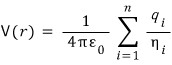

Using the same zero at infinity for all contributions, we can write this as

$$ V(\mathbf r)=\frac{1}{4\pi\epsilon_0}\sum_{i=1}^{n}\frac{q_i}{|\mathbf r-\mathbf r_i|}. $$

The observation point must be different from every source point, so each distance in the denominator is positive.

What about a continuous charge distribution?

Then the sum becomes an integral. That was my quick answer in the original note, and the idea is exactly the same: add the potential contributed by each small bit of charge.

For a localized distribution with a well-defined integral and zero potential at infinity,

$$ V(\mathbf r)=\frac{1}{4\pi\epsilon_0}\int\frac{dq(\mathbf r')}{|\mathbf r-\mathbf r'|}. $$

The primed coordinate $\mathbf r'$ labels the source being integrated over; $\mathbf r$ stays fixed at the observation point. The small charge $dq$ keeps its sign. For a volume charge density,

$$ dq=\rho(\mathbf r')\,d^3\mathbf r'. $$

So the move from separate charges to a continuous distribution really is a move from a sum to an integral, with the same source-to-observer distance in each contribution.