Electrostatics in Conductors: Surface Charge and Potential

A conductor contains mobile charge carriers. In a metal, conduction electrons can redistribute when an electric field acts on them. That freedom makes electrostatic problems much simpler: first find the charge distribution consistent with equilibrium, then use it to calculate the field and potential.

Here we use the classical, macroscopic model of an ideal conductor in electrostatic equilibrium, after charge redistribution has finished. There is no sustained current or imposed electromotive force. A real good conductor approximates this behavior after its initial transients have died away.

Why the field vanishes in the metal

If a nonzero electric field remained in the conducting material, it would drive its mobile charges. The distribution would still be changing. Equilibrium therefore requires

$$ \mathbf E=\mathbf 0 \qquad\text{in the metal}. $$

Imagine giving a solid, isolated conductor a net charge $q$. The first sketch represents an initial charge placement; a localized excess charge in the bulk cannot remain there at equilibrium. The red plus signs illustrate the case $q>0$. In a metal, positive excess charge means an electron deficit, not positive lattice ions migrating outward.

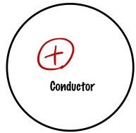
The mobile electrons rearrange until the field in the metal vanishes. In the continuum model, the excess charge then resides on the external surface. Its surface density need not be uniform for an arbitrary shape or in an external field.

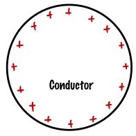
The marked point $r$ in the next sketch is in the conducting material, so the equilibrium field there is zero.

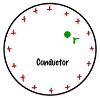
Gauss’s law now tells us something about the charge in the bulk. Choose a closed Gaussian surface lying wholly in the metal, as sketched in blue.

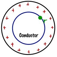
With $d\mathbf A$ directed outward, the electric flux is

$$ \oint_S\mathbf E\cdot d\mathbf A =\frac{Q_{\mathrm{enc}}}{\epsilon_0}=0. $$

Thus every small volume wholly within the metal has zero net macroscopic charge. Equivalently, the bulk charge density is $\rho=0$. Electrons and positive lattice ions are still present; their charges cancel in this macroscopic description.

The order of the argument matters. Equilibrium gives a zero field, and Gauss’s law then gives zero net bulk charge. Zero enclosed charge alone would give only zero net flux. For example, a uniform nonzero field also has zero flux through a closed sphere.

A sphere of radius $k$ has area $4\pi k^2$. When spherical symmetry makes the field radial and its radial component constant on that sphere, the flux simplifies to

$$ \oint_S\mathbf E\cdot d\mathbf A =4\pi k^2 E_r(k). $$

That simplification needs the stated symmetry; merely choosing a spherical Gaussian surface does not establish it. The equilibrium and bulk-charge arguments are also explained in Richard Fitzpatrick’s Ideal Conductors.

Induction and cavities

A nearby charge can redistribute the electrons in an initially neutral conductor, producing regions of positive and negative surface charge. This is electrostatic induction. An isolated conductor remains neutral overall unless charge is supplied or removed. Connecting it to ground would permit charge exchange and change the problem.

Zero field in the metal does not mean zero field everywhere within its outer boundary. A charge in a cavity can produce a field in the cavity and induce charge on its internal wall, while the surrounding metal still has zero field. A completely enclosed, charge-free cavity has zero electrostatic field; the gap surrounding a charged inner conductor in the example below is a different situation. OpenStax discusses these distinctions in Conductors in Electrostatic Equilibrium.

A sphere inside a neutral conducting shell

Let’s work through a problem. A solid conducting sphere of radius $R$ carries a fixed signed net charge $q$. A concentric conducting shell occupies $a\lt r\lt b$, with

$$ 0\lt R\lt a\lt b. $$

The shell is initially neutral, isolated, and ungrounded. The gap and exterior are vacuum, there is no external field, and we choose $V(\infty)=0$. The coordinate $r$ now denotes distance from the common center. We want the potential at that center.

The next four sketches build up the charge distribution in stages. They are bookkeeping diagrams, not four separate equilibrium states; only the last shows the complete final distribution. The central charge label in the first sketch indicates the inner sphere’s net charge, not a deposit that remains at its center.

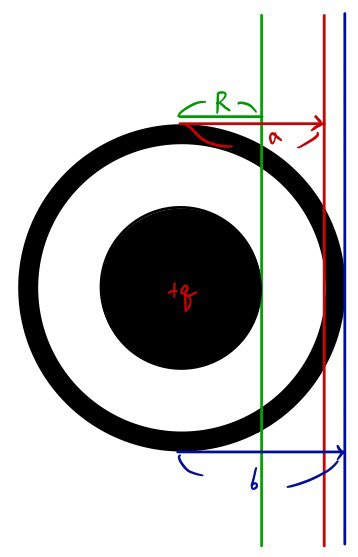
At equilibrium, the inner sphere’s charge lies on its surface at $r=R$. The sketches show $q>0$; reversing the sign of $q$ reverses the induced signs and electric-field direction.

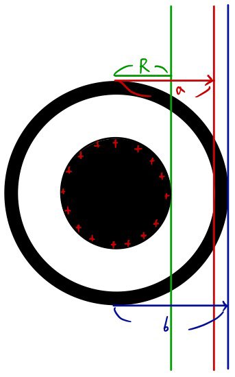
Let $q_a$ and $q_b$ denote the charges on the shell’s inner and outer surfaces. A Gaussian sphere with $a\lt r\lt b$ lies in metal, where the field is zero. It encloses the inner sphere and the shell’s inner surface, so Gauss’s law gives

$$ q+q_a=0, \qquad q_a=-q. $$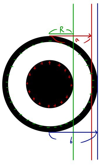

The isolated shell has zero net charge. Charge conservation therefore supplies the second constraint:

$$ q_a+q_b=0, \qquad q_b=q. $$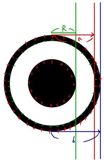

Concentric spherical symmetry and the absence of an external field make the charge density uniform on each surface. Dividing each charge by its corresponding area gives the three densities shown here.

Thus $\sigma_R=q/(4\pi R^2)$, $\sigma_a=-q/(4\pi a^2)$, and $\sigma_b=q/(4\pi b^2)$. These are local densities here because of symmetry; charge divided by total area gives only an average in a general geometry.

The electric field in four regions

Spherical symmetry lets us write the field away from the origin as

$$ \mathbf E(r)=E_r(r)\,\hat{\mathbf r}, $$

where $\hat{\mathbf r}$ points outward. The signed radial component is $E_r$: it is positive for an outward field and negative for an inward one. The scalar $E$ in the two retained equation images below has this radial meaning.

Outside the shell, a Gaussian sphere encloses the total charge $q+q_a+q_b=q$. Its flux is $4\pi r^2E_r(r)$, giving

$$ E_r(r)=\frac{q}{4\pi\epsilon_0 r^2}, \qquad r>b. $$

Within the shell’s metal, equilibrium gives

$$ E_r(r)=0, \qquad a\lt r\lt b. $$

In the vacuum gap, a Gaussian sphere encloses only the inner sphere’s charge. Hence

$$ E_r(r)=\frac{q}{4\pi\epsilon_0 r^2}, \qquad R\lt r\lt a. $$

Finally, inside the solid inner conductor,

$$ E_r(r)=0, \qquad 0\lt r\lt R. $$

At the origin itself, the field is the zero vector; no radial direction needs to be assigned there. We use strict inequalities at the charged surfaces because the electric field has distinct one-sided limits. The potential remains continuous across each surface.

Integrating the potential to the center

Starting from the reference $V(\infty)=0$, integrate inward along a radial path. Use $s$ as the integration variable. The path crosses the exterior, the shell’s metal, the vacuum gap, and the solid inner conductor:

$$ \begin{aligned} V(0)={}&-\int_{\infty}^{b}E_r(s)\,ds\\ &-\int_b^a 0\,ds\\ &-\int_a^R E_r(s)\,ds\\ &-\int_R^0 0\,ds. \end{aligned} $$

The two metal intervals contribute zero potential difference. Substituting the field in the other two intervals and keeping the leading minus sign gives

$$ \begin{aligned} V(0)&=-\frac{q}{4\pi\epsilon_0}\\ &\quad\times\left\{ \left[-\frac1s\right]_{\infty}^{b} +\left[-\frac1s\right]_{a}^{R} \right\}. \end{aligned} $$

The first bracket is $-1/b$ and the second is $-1/R+1/a$. Therefore

$$ V(0)=\frac{q}{4\pi\epsilon_0} \left(\frac1R-\frac1a+\frac1b\right). $$

Since the field vanishes throughout the inner metal, its entire volume and surface share this value: $V(R)=V(0)$. The shell is also an equipotential, with

$$ V(a)=V(b)=\frac{q}{4\pi\epsilon_0 b}. $$

The two disconnected conductors can have different constant potentials. In fact, their potential difference is

$$ V(R)-V(a)=\frac{q}{4\pi\epsilon_0} \left(\frac1R-\frac1a\right). $$

This is the useful distinction: a zero electric field makes the potential constant within a conductor. It does not require that constant to be zero. An absolute value follows only after we choose a reference, as we did at infinity.

Editorial note — 9 September 2026

This English edition restores the intended image sequence from the original Korean post and translates the four conductor labels. It also corrects the original flux argument: equilibrium establishes the zero field, and a spherical surface contributes area $4\pi k^2$, not volume. A missing intermediate minus sign in the potential derivation has been corrected; the original final expression for $V(0)$ was already correct. The two faulty displayed derivations have been replaced with accessible TeX, while the historical image files are preserved. The assumptions and the role of the successive charge sketches are made explicit above.