Multipole Expansion

What is a multipole expansion?

I had just encountered it when I wrote the original post, and the basic idea is surprisingly intuitive. A localized charge distribution viewed from far away can often be described by a sequence of progressively finer terms: monopole, dipole, quadrupole, and so on. If the total charge is nonzero, the monopole term usually dominates the far field. If it vanishes, the first nonzero higher moment takes over.

Starting with a finite dipole

Consider two charges, \(+q\) and \(-q\), separated by a displacement of magnitude \(d\).

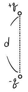
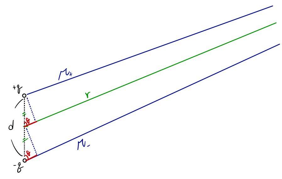
Place the charges at \(\pm (d/2)\hat{\mathbf z}\), and let the observation point be \(\mathbf r\), with \(r=|\mathbf r|\) and polar angle \(\theta\).

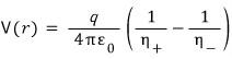
The exact potential is the sum of the two point-charge potentials:

The exact source-to-field-point distances are

\[ R_+=\sqrt{r^2+\frac{d^2}{4}-rd\cos\theta}, \qquad R_-=\sqrt{r^2+\frac{d^2}{4}+rd\cos\theta}. \]

For \(r\gg d\), their first-order projected-distance approximations are

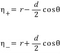
or \(R_+\approx r-(d/2)\cos\theta\) and \(R_-\approx r+(d/2)\cos\theta\). Substituting these approximations gives

\[ \begin{aligned} V(r,\theta) &\approx \frac{q}{4\pi\epsilon_0} \left[ \frac{1}{r-(d/2)\cos\theta} -\frac{1}{r+(d/2)\cos\theta} \right] \\ &=\frac{1}{4\pi\epsilon_0} \frac{qd\cos\theta}{r^2-(d^2/4)\cos^2\theta} \\ &\approx \frac{1}{4\pi\epsilon_0}\frac{p\cos\theta}{r^2}, \qquad p=qd, \end{aligned} \]

where the last line keeps the leading term for \(r\gg d\).

Source correction. The source image at this point prints a plus sign in the projected-distance denominator. The corrected denominator is \(r^2-(d^2/4)\cos^2\theta\), as shown above.

The pattern is now visible. A monopole contribution scales as \(r^{-1}\), a dipole contribution as \(r^{-2}\), a quadrupole contribution as \(r^{-3}\), and an octupole contribution as \(r^{-4}\). These statements describe the radial order at a fixed direction where the relevant angular factor is nonzero. An angular node of the potential does not mean that the whole multipole moment—or even the electric field—vanishes there.

For the centered \(+q,-q\) pair above, inversion symmetry makes the charge distribution odd. Its even-\(\ell\) contributions cancel, but odd orders beyond the dipole, such as \(\ell=3,5,\ldots\), can still remain. Calling it a “dipole” identifies its leading nonzero moment, not the only term in the exact finite-separation potential.

A general localized charge distribution

Now consider a continuous charge distribution confined to a finite region.

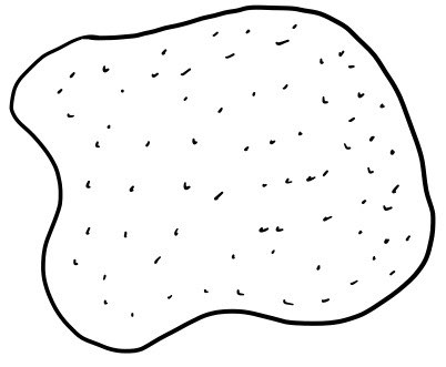
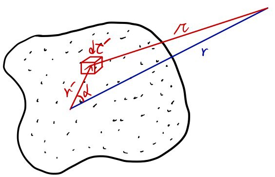
Let \(\mathbf r\) be the observation point and \(\mathbf r'\) a source point. Define

\[ \mathbf R=\mathbf r-\mathbf r',\qquad R=|\mathbf R|,\qquad r=|\mathbf r|,\qquad r'=|\mathbf r'|, \]

and let \(\alpha\) be the angle between \(\mathbf r\) and \(\mathbf r'\), so that \(\cos\alpha=\hat{\mathbf r}\cdot\hat{\mathbf r}'\).

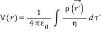
The electrostatic potential is

and the geometry gives

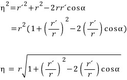
that is,

\[ R^2=r^2+r'^2-2rr'\cos\alpha. \]

Set \(t=r'/r\). The Legendre generating function gives

\[ \frac{1}{R} =\frac{1}{r}\left(1-2t\cos\alpha+t^2\right)^{-1/2} =\frac{1}{r}\sum_{\ell=0}^{\infty}t^\ell P_\ell(\cos\alpha), \qquad r'\lt r. \]

For a source contained inside \(r'\le a\), this exterior expansion applies for \(r>a\). On any region \(r\ge r_0>a\), the series converges uniformly enough to justify term-by-term integration.

If one reaches the result through the binomial series, it is important not to stop too soon. With \(u=t^2-2t\cos\alpha\), a derivation through \(P_3\) needs the \(-5u^3/16\) term; the displayed \(u^0\), \(u^1\), and \(u^2\) terms alone do not produce the full cubic coefficient. The Legendre generating function is also the clean way to state the full domain \(|t|<1\); the intermediate condition \(|u|<1\) can be unnecessarily restrictive.

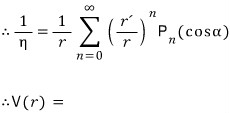
The first few terms are

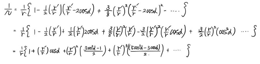
so the coefficient of \(t^\ell\) is \(P_\ell(\cos\alpha)\). Substituting the series into the potential produces

\[ V(\mathbf r) =\frac{1}{4\pi\epsilon_0} \sum_{\ell=0}^{\infty}\frac{1}{r^{\ell+1}} \int r'^\ell P_\ell(\cos\alpha)\rho(\mathbf r')\,d\tau'. \]

The first three orders are

\[ V(\mathbf r)=\frac{1}{4\pi\epsilon_0} \left[ \frac{Q}{r} +\frac{1}{r^2}\int r'\cos\alpha\,\rho(\mathbf r')\,d\tau' +\frac{1}{r^3}\int \frac{r'^2}{2}\left(3\cos^2\alpha-1\right) \rho(\mathbf r')\,d\tau' +\cdots \right], \]

with \(Q=\int\rho(\mathbf r')\,d\tau'\).

Source correction. The source image uses \(r'^2\) in the general \(\ell\) term and gives an incorrect power and angular factor in the quadrupole term. The equations above restore \(r'^\ell\) generally and \(r'^2(3\cos^2\alpha-1)/2\) at \(\ell=2\).

For a fixed source distribution and a fixed origin, the multipole moments are fixed. Moving the observer changes \(r\) and the angular factors at which the expansion is evaluated; it does not change the source moments themselves. If the \(z\)-axis is chosen along \(\mathbf r\), then \(\alpha\) is the source point’s polar angle \(\theta'\). Later, when the \(z\)-axis is chosen along \(\mathbf p\), the \(\theta\) in \(p\cos\theta\) is the observation angle. Those are different coordinate choices.

The far-field hierarchy is controlled by the lowest nonzero moment, but only away from its angular nodes. When \(Q\ne0\), the monopole term is normally leading. When \(Q=0\), the dipole term leads only if the dipole moment is nonzero.

The dipole moment

The dipole term can be written using

\[ \mathbf p=\int \mathbf r'\rho(\mathbf r')\,d\tau', \qquad V_{\mathrm{dip}}(\mathbf r) =\frac{1}{4\pi\epsilon_0}\frac{\mathbf p\cdot\hat{\mathbf r}}{r^2}. \]

Source correction. The corresponding source image omits the explicit scalar-product dot in its last expression. It is restored here because the potential is a scalar.

For discrete point charges,

or \(\mathbf p=\sum_i q_i\mathbf r_i'\).

Return to a pair of charges \(-q\) and \(+q\).

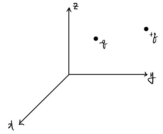
Let \(\mathbf r_1'\) point from the origin to \(-q\), and \(\mathbf r_2'\) point from the origin to \(+q\). Define the displacement from the negative charge to the positive charge by

\[ \mathbf d=\mathbf r_2'-\mathbf r_1'. \]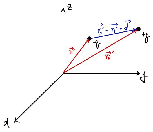

Then

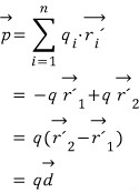
so \(\mathbf p=q\mathbf d\).

When the dipole moment also vanishes

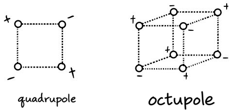
A neutral distribution need not have a nonzero dipole moment. With equal-magnitude charges at centered symmetric positions, an alternating-charge square has \(Q=0\) and \(\mathbf p=0\), while a quadrupole component remains. Likewise, the centered alternating cube shown below cancels all orders below \(\ell=3\), leaving an octupole as its leading moment. Finite arrangements can still contain higher moments beyond the leading one.

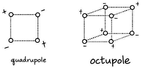
This is why “the first nonzero multipole” is the useful phrase: symmetry may eliminate one or several lower orders.

Dependence on the choice of origin

There is one more important detail: multipole moments are coordinates of a source relative to a chosen origin.

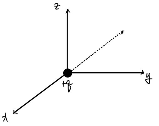
For a point charge at the origin, the discrete definition

gives zero dipole moment.

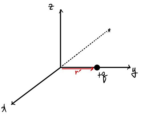
If the origin is shifted by a vector \(\mathbf a\), so that \(\mathbf r'_{\mathrm{new}}=\mathbf r'_{\mathrm{old}}-\mathbf a\), then

\[ \mathbf p_{\mathrm{new}}=\mathbf p_{\mathrm{old}}-Q\mathbf a. \]

Therefore the dipole moment is origin-independent when \(Q=0\), but not in general. This coordinate dependence of individual moments does not change the physical potential or electric field when the whole expansion and coordinates are transformed consistently.

Electric field of an ideal dipole

Choose the \(z\)-axis along \(\mathbf p=p\hat{\mathbf z}\), and use spherical coordinates for an observation point away from the source.

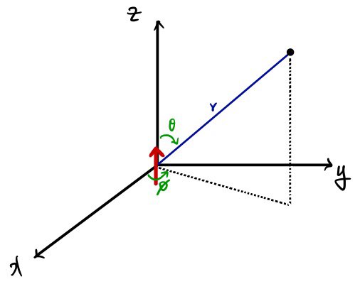
For \(r>0\), the ideal-dipole potential is

\[ V_{\mathrm{dip}}(r,\theta) =\frac{1}{4\pi\epsilon_0} \frac{\mathbf p\cdot\hat{\mathbf r}}{r^2} =\frac{1}{4\pi\epsilon_0}\frac{p\cos\theta}{r^2}. \]

It is independent of the azimuthal angle \(\phi\). Taking \(\mathbf E=-\nabla V\) gives

\[ \mathbf E(r,\theta) =\frac{p}{4\pi\epsilon_0 r^3} \left(2\cos\theta\,\hat{\mathbf r} +\sin\theta\,\hat{\boldsymbol\theta}\right), \qquad E_\phi=0, \qquad r>0. \]

Source correction. The source image omits \(p\) from its first displayed radial component. The corrected field above includes it. The ideal-dipole expression is not defined at \(r=0\).

That completes the basic picture: expand the inverse distance in Legendre polynomials, integrate each angular order against the source, and let the first nonzero moment describe the leading far field.

References

• MIT OpenCourseWare 8.07, Lecture Notes 9: Multipole expansion
• University of Illinois Physics 435, Lecture 8: Electric dipoles and fields
• related note