Polarization

From here on, we are studying electrostatic fields inside matter.

In the preceding chapters, we mostly worked in vacuum, so we used the vacuum permittivity \(\varepsilon_0\) without having to discuss how a material responds. Inside water, a solid dielectric, or a gas, the charges in the material respond to an applied electric field. That response changes the resulting electric field and potential.

Let us begin with a neutral atom placed in an external electric field \(\mathbf E\).

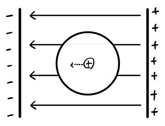
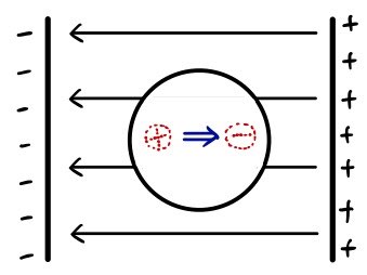
The field shifts the positive nucleus slightly in one direction and the negative electron cloud slightly in the other. The separated charges create an internal field that opposes the displacement. Unless the applied field is so strong that the atom is ionized or driven outside the linear regime, the two effects settle into equilibrium.

The blue arrow in the retained source drawing is unlabeled and points from the positive side toward the negative side. It must not be read as \(\mathbf p\): by convention, the electric dipole moment points from negative charge toward positive charge, parallel to the applied field in this drawing.

We say that the atom has been polarized. It now carries a small induced dipole moment \(\mathbf p\). In the simplest isotropic, linear-response approximation,

\[ \mathbf p=\alpha\mathbf E_{\mathrm{loc}} \qquad\text{(isotropic, linear-response approximation)} \]

Here \(\mathbf E_{\mathrm{loc}}\) is the local field acting on the atom and \(\alpha\) is the atomic polarizability. Different atoms have different polarizabilities: the same local field produces a larger displacement in some atoms than in others. More generally, \(\alpha\) is a tensor and \(\mathbf p=\boldsymbol\alpha\cdot\mathbf E_{\mathrm{loc}}\).

For this discussion, it is enough to know what \(\alpha\) measures. A complete microscopic calculation belongs to quantum mechanics, not this classical macroscopic model. (You could spend 218371273981279 hours trying to follow every microscopic detail classically, but that would miss the point.)

From atomic dipoles to polarization density

Now replace the single atom with a piece of dielectric containing many atoms. The applied field polarizes the atoms, so the material acquires a dipole moment throughout its volume.

We describe this collectively by the polarization field

\[ \mathbf P(\mathbf r') =\frac{\text{dipole moment in a small volume around }\mathbf r'} {\text{that volume}}. \]

Thus \(\mathbf P\) is dipole moment per unit volume, and it is a vector.

Imagine that the dielectric has been polarized and that, for the moment, the polarization remains after the external field is removed. Some materials lose their polarization when the field disappears; the retained-polarization picture here is simply the configuration whose field we want to calculate.

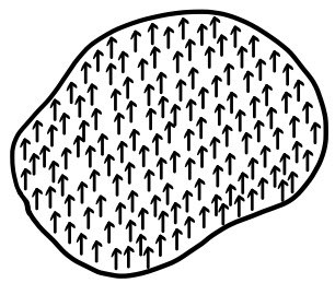
For a uniformly polarized example, all the little dipole moments point the same way.

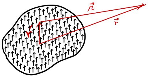
Let \(\mathbf r'\) locate a source element inside the dielectric, let \(\mathbf r\) locate the observation point, and define

\[ \boldsymbol\eta=\mathbf r-\mathbf r', \qquad \eta=|\boldsymbol\eta|. \]

What potential does the polarized object produce at \(\mathbf r\)? We add the contributions from all its infinitesimal dipoles.

For one dipole \(\mathbf p\) at \(\mathbf r'\), the potential at \(\mathbf r\) is

\[ V_{\mathrm{dip}}(\mathbf r;\mathbf r') =\frac{1}{4\pi\varepsilon_0} \frac{\mathbf p\cdot(\mathbf r-\mathbf r')}{|\mathbf r-\mathbf r'|^3} =\frac{1}{4\pi\varepsilon_0} \frac{\mathbf p\cdot\widehat{\boldsymbol\eta}}{\eta^2}, \qquad \boldsymbol\eta\equiv\mathbf r-\mathbf r'. \]

Source correction. The original prose writes the shorthand \(V(r)=pr/(4\pi\varepsilon)\). That expression omits the vector dot product and the required inverse powers of separation. The equation above gives the complete point-dipole potential used by the following integral.

Because a source volume \(d^3r'\) carries dipole moment \(d\mathbf p=\mathbf P(\mathbf r')d^3r'\), integration gives

\[ V_{\mathrm{pol}}(\mathbf r) =\frac{1}{4\pi\varepsilon_0} \int_V \frac{\mathbf P(\mathbf r')\cdot\widehat{\boldsymbol\eta}}{\eta^2}\,d^3r', \qquad \boldsymbol\eta=\mathbf r-\mathbf r',\quad \eta=|\boldsymbol\eta|. \]

Rewriting the potential as bound-charge contributions

The sign depends on which coordinate the gradient differentiates. With \(\nabla'\) acting on the source coordinate \(\mathbf r'\), while \(\nabla\) acts on the observation coordinate \(\mathbf r\),

\[ \nabla'\!\left(\frac{1}{\eta}\right) =\frac{\boldsymbol\eta}{\eta^3} =\frac{\widehat{\boldsymbol\eta}}{\eta^2} =-\nabla\!\left(\frac{1}{\eta}\right), \qquad \boldsymbol\eta=\mathbf r-\mathbf r'. \]

Keep \(\mathbf P=\mathbf P(\mathbf r')\) for the general derivation. The product rule and divergence theorem give

\[ \begin{aligned} V_{\mathrm{pol}}(\mathbf r) &=\frac{1}{4\pi\varepsilon_0} \int_V \mathbf P(\mathbf r')\cdot\nabla'\!\left(\frac{1}{\eta}\right)\,d^3r'\\ &=\frac{1}{4\pi\varepsilon_0} \int_V\left[ \nabla'\cdot\!\left(\frac{\mathbf P(\mathbf r')}{\eta}\right) -\frac{\nabla'\cdot\mathbf P(\mathbf r')}{\eta} \right]d^3r'\\ &=\frac{1}{4\pi\varepsilon_0} \oint_{\partial V} \frac{\mathbf P(\mathbf r')\cdot\hat{\mathbf n}'}{\eta}\,da' -\frac{1}{4\pi\varepsilon_0} \int_V \frac{\nabla'\cdot\mathbf P(\mathbf r')}{\eta}\,d^3r'. \end{aligned} \]

Here \(\hat{\mathbf n}'\) is the outward unit normal on the boundary \(\partial V\) of the polarized body. Define the bound surface and volume charge densities by

\[ \sigma_b(\mathbf r')=\mathbf P(\mathbf r')\cdot\hat{\mathbf n}', \qquad \rho_b(\mathbf r')=-\nabla'\cdot\mathbf P(\mathbf r'). \]

The surface density is positive where \(\mathbf P\) points outward and negative where it points inward. The minus sign in \(\rho_b=-\nabla\cdot\mathbf P\) is essential.

The potential can therefore be written as

\[ V_{\mathrm{pol}}(\mathbf r) =\frac{1}{4\pi\varepsilon_0} \left[ \oint_{\partial V} \frac{\sigma_b(\mathbf r')}{|\mathbf r-\mathbf r'|}\,da' +\int_V \frac{\rho_b(\mathbf r')}{|\mathbf r-\mathbf r'|}\,d^3r' \right]. \]

This is the central result: a polarized object produces the same potential as a bound surface charge density \(\sigma_b\) together with a bound volume charge density \(\rho_b\).

You can picture polarization as a large collection of slightly separated positive and negative charges. In the interior, neighboring dipoles mostly cancel. A net charge can remain where \(\mathbf P\) changes through the volume or where the material ends.

If \(\mathbf P\) is uniform in the material bulk, then \(\nabla\cdot\mathbf P=0\) there and \(\rho_b=0\) in the bulk. The surface charge generally remains because \(\mathbf P\) jumps to zero outside the material, leaving \(\sigma_b=\mathbf P\cdot\hat{\mathbf n}\) on the boundary.

So why exactly do the effective charges take these forms? Here is the same definition once more, matching the original post’s deliberate recap:

\[ \sigma_b(\mathbf r')=\mathbf P(\mathbf r')\cdot\hat{\mathbf n}', \qquad \rho_b(\mathbf r')=-\nabla'\cdot\mathbf P(\mathbf r'). \]

Honestly, this part was very difficult for me when I first studied it. I formed a working picture and kept going, but it still felt rough. In the next post, I will derive these bound-charge relations more directly.