Bound Charge Density

In the previous post on polarization, we found that a polarized dielectric next to vacuum can be described by two kinds of bound charge:

\[ \sigma_b=\mathbf P\cdot\hat{\mathbf n}, \qquad \rho_b=-\nabla\cdot\mathbf P. \]

Here the first formula refers to the material’s physical boundary, with \(\hat{\mathbf n}\) directed outward into the vacuum. I spent a long time trying to make these two compact formulas feel intuitive. The picture I eventually settled on was useful, but it needed one important correction: polarization is not itself an amount of charge.

What polarization measures

The polarization field \(\mathbf P\) is electric dipole moment per unit volume. Its SI units are therefore

\[ [\mathbf P] =\frac{\mathrm{C\,m}}{\mathrm{m^3}} =\mathrm{C/m^2}. \]

That happens to be the same unit as surface charge density, but the two quantities are not interchangeable. \(\mathbf P\) is a vector field that records both the strength and direction of the local dipole moment density. The scalar \(\sigma_b\) is the bound charge per unit area on a physical interface, and it depends on the polarization on both sides and on the chosen normal.

My first mental picture was a tiny volume containing equal and opposite charges displaced along \(\mathbf P\). That is a good way to remember the dipole structure. It is not correct, however, to say that \(|\mathbf P|\) is simply a charge \(q\) piled on one side of a unit volume. The dimensions already warn us: \(|\mathbf P|\) is measured in \(\mathrm{C/m^2}\), not coulombs.

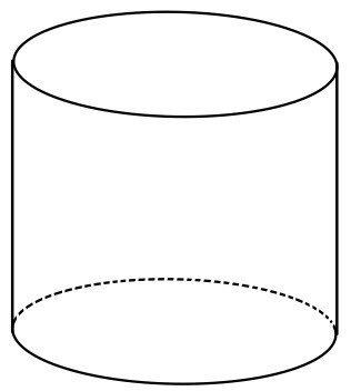
Suppose this small cylinder is uniformly polarized. Neighboring microscopic dipoles cancel through most of the interior, leaving opposite bound charges exposed on its end faces.

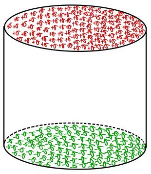
Why the surface charge is \(\mathbf P\cdot\hat{\mathbf n}\)

First take a right prism whose axis is parallel to a uniform polarization \(\mathbf P\). Let its length be \(\ell\), and let an end face perpendicular to \(\mathbf P\) have area \(S_\perp\). Choose the positive end face, whose outward normal points along \(\mathbf P\), and call its positive bound charge \(Q_+\). The dipole moment of the prism is \(Q_+\ell\). Dividing by its volume \(S_\perp\ell\) gives

\[ P=\frac{Q_+\ell}{S_\perp\ell} =\frac{Q_+}{S_\perp}. \]

Thus \(Q_+=P S_\perp\) on the positive face. The opposite face carries the signed charge \(Q_-=-Q_+\). This is the precise version of the intuition that the magnitude of \(\mathbf P\) can look like a surface charge density: it is true on a perpendicular face, while the outward normal determines the sign.

Now cut the polarized cylinder at an angle.

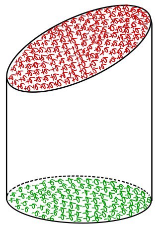
Let \(S\) be the area of a slanted physical boundary face, and let \(\theta\) be the angle between \(\mathbf P\) and its outward unit normal \(\hat{\mathbf n}\). The ordinary, unsigned projected area perpendicular to \(\mathbf P\) is

\[ S_{\mathrm{proj}}=S|\cos\theta|, \qquad |Q_b|=P S_{\mathrm{proj}}=P S|\cos\theta|. \]

If \(Q_b\) denotes the signed charge on that face, the orientation supplies the sign:

\[ Q_b=P S\cos\theta, \qquad \sigma_b=\frac{Q_b}{S} =P\cos\theta =\mathbf P\cdot\hat{\mathbf n}. \]

Where \(\mathbf P\) points outward, \(Q_b\) and \(\sigma_b\) are positive; where it points inward, they are negative; and where \(\mathbf P\) lies tangent to the interface, they vanish. The absolute value in the projected-area formula and the signed dot product are therefore consistent even when \(\theta>\pi/2\).

This one-sided formula applies when the polarized material meets vacuum, or more generally when the polarization on the other side is zero. At an interface between two polarized media, define \(\hat{\mathbf n}\) to point from the “in” side to the “out” side. The general bound sheet charge is the jump in normal polarization:

\[ \boxed{ \sigma_b=(\mathbf P_{\mathrm{in}}-\mathbf P_{\mathrm{out}}) \cdot\hat{\mathbf n} }. \]

For a material-vacuum boundary, \(\mathbf P_{\mathrm{out}}=0\), so this reduces to

\[ \sigma_b=\mathbf P_{\mathrm{in}}\cdot\hat{\mathbf n}. \]

The signed bound charge on a patch \(A\) of that physical boundary is

\[ Q_b(A)=\int_A \sigma_b\,da. \]

An imaginary surface drawn inside a smooth material does not acquire an actual bound-charge sheet. On such a control surface, \(\mathbf P\cdot\hat{\mathbf n}\) is instead a polarization-flux integrand used to account for the volume charge enclosed.

Why the volume charge is \(-\nabla\cdot\mathbf P\)

The second relation describes bound charge distributed through the material:

\[ \rho_b=-\nabla\cdot\mathbf P. \]

Here \(\rho_b\) is bound volume charge density, measured in \(\mathrm{C/m^3}\). For a region \(V\) inside the material,

\[ Q_{b,\mathrm{vol}}(V)=\int_V \rho_b\,d\tau. \]

It is tempting to argue that every charge inside has an opposite partner just outside. That picture is too literal: there is no general point-by-point pairing across an arbitrary boundary. What matters is the net imbalance of dipole ends enclosed by a small control volume.

For an arbitrary control volume \(V\) lying in a smoothly polarized region, the outward polarization flux accounts for that imbalance. A positive outward flux corresponds to a deficit of positive bound charge inside, so

\[ Q_{b,\mathrm{vol}}(V) =-\oint_{\partial V}\mathbf P\cdot\hat{\mathbf n}\,da. \]

The integrand here is flux through an imaginary control boundary, not a claim that \(\partial V\) carries a physical charge sheet. Applying the divergence theorem gives

\[ \int_V \rho_b\,d\tau =-\oint_{\partial V}\mathbf P\cdot\hat{\mathbf n}\,da =-\int_V \nabla\cdot\mathbf P\,d\tau. \]

Because this holds for every sufficiently small control volume in the smooth bulk, the integrands must agree locally:

\[ \boxed{\rho_b=-\nabla\cdot\mathbf P}. \]

This is the local argument. It does not depend on matching an inside charge to an outside charge at each point.

Bulk charge and surface charge are complementary

If \(\mathbf P\) is uniform throughout the bulk, then \(\nabla\cdot\mathbf P=0\), so there is no bound volume charge there. The drawings above show the remaining bound charge on the material’s physical surface, where the polarized material ends and \(\mathbf P\) changes to zero outside.

For one polarized body occupying \(V\) and surrounded by vacuum, we keep the two contributions distinct:

\[ Q_{b,\mathrm{vol}}=\int_V \rho_b\,d\tau, \qquad Q_{b,\mathrm{surf}}=\oint_{\partial V}\sigma_b\,da. \]

Using the two local definitions,

\[ \begin{aligned} Q_{b,\mathrm{vol}}+Q_{b,\mathrm{surf}} &=-\int_V \nabla\cdot\mathbf P\,d\tau +\oint_{\partial V}\mathbf P\cdot\hat{\mathbf n}\,da\\ &=0, \end{aligned} \]

for a complete localized polarized body with a sufficiently regular polarization field. This global cancellation is a consequence of the divergence theorem. It should not be mistaken for a naive pointwise pairing of charges on the two sides of every imagined surface.

The picture I keep is now more precise: polarization is dipole moment per unit volume. Its jump in the normal direction produces a bound sheet charge at a physical interface, while spatial convergence or divergence of \(\mathbf P\) produces bound volume charge in the bulk.