Linear Dielectrics

We introduced the dipole moment of an atom or molecule through a relation such as

\[ \mathbf p=\alpha\mathbf E_{\mathrm{local}}, \]

where \(\alpha\) is the atomic or molecular polarizability. A larger \(\alpha\) means that the same local electric field induces a larger dipole moment.

For a macroscopic material, tracking every microscopic dipole is impractical. Instead we use the polarization \(\mathbf P\), the electric dipole moment per unit volume. In a simple isotropic linear dielectric, the macroscopic constitutive relation is

\[ \boxed{\mathbf P=\varepsilon_0\chi_e\mathbf E}, \]

where \(\chi_e\) is the dimensionless electric susceptibility and \(\mathbf E\) is the total macroscopic electric field in the material. The factor \(\varepsilon_0\) is included so that \(\chi_e\) has no units.

This scalar relation assumes a linear, isotropic medium. If the material is anisotropic, susceptibility is generally a tensor; if its response is nonlinear, \(\mathbf P\) is not simply proportional to \(\mathbf E\). Both \(\chi_e\) and the resulting permittivity can also depend on temperature and, for time-dependent fields, frequency.

Susceptibility, permittivity, and the displacement field

The electric displacement field is defined by

\[ \mathbf D=\varepsilon_0\mathbf E+\mathbf P. \]

Substituting the linear constitutive relation gives

\[ \mathbf D =\varepsilon_0\mathbf E+\varepsilon_0\chi_e\mathbf E =\varepsilon_0(1+\chi_e)\mathbf E =\varepsilon\mathbf E, \]

with

\[ \boxed{\varepsilon=\varepsilon_0(1+\chi_e)}. \]

So \(\chi_e\) measures how strongly the material polarizes, while \(\varepsilon\) connects \(\mathbf D\) to the total macroscopic field \(\mathbf E\) in this isotropic linear medium.

In electrostatics,

\[ \nabla\cdot\mathbf D=\rho_f, \qquad \oint_S\mathbf D\cdot d\mathbf a=Q_{f,\mathrm{enc}}. \]

This is why \(\mathbf D\) is so useful: its flux is determined by free charge, while polarization is absorbed into the constitutive relation. But \(\mathbf D\) should not be described as “the electric field produced by free charge.” It is an auxiliary field, and the physical electric field is still \(\mathbf E\).

For a fixed free-charge distribution in a simple geometry, a larger \(\varepsilon\) produces a smaller \(\lvert\mathbf E\rvert=\lvert\mathbf D\rvert/\varepsilon\) inside the dielectric. That reduction is the macroscopic effect of the bound charges created by polarization.

Example: conducting sphere with a dielectric shell

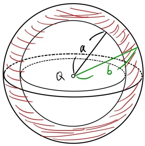
A conducting sphere of radius \(a\) carries total free charge \(Q\). A homogeneous, isotropic, linear dielectric of permittivity \(\varepsilon\) fills the concentric shell from \(r=a\) to \(r=b\). The region outside the shell is vacuum. Find \(\mathbf D\), \(\mathbf E\), the potential \(V\), and the bound charges.

We assume electrostatic equilibrium, spherical symmetry, and \(V(\infty)=0\). The free charge lies on the conductor surface. There is no additional free charge in the dielectric or at its outer boundary.

Displacement field

Inside the conductor, the electrostatic field vanishes. For a spherical Gaussian surface with \(r\gt a\), the enclosed free charge is \(Q\), so

\[ 4\pi r^2D_r=Q. \]

Therefore

\[ \boxed{ \mathbf D(r)= \begin{cases} \mathbf 0, & 0\le r\lt a,\\[4pt] \displaystyle\frac{Q}{4\pi r^2}\,\hat{\mathbf r}, & r\gt a. \end{cases}} \]

At \(r=a\), the normal component jumps by the free surface-charge density

\[ \sigma_f=\frac{Q}{4\pi a^2}. \]

At \(r=b\), there is no free surface charge, so the normal component of \(\mathbf D\) is continuous.

Electric field

Use \(\mathbf D=\varepsilon\mathbf E\) in the dielectric and \(\mathbf D=\varepsilon_0\mathbf E\) in vacuum:

\[ \boxed{ \mathbf E(r)= \begin{cases} \mathbf 0, & 0\le r\lt a,\\[4pt] \displaystyle\frac{Q}{4\pi\varepsilon r^2}\,\hat{\mathbf r}, & a\lt r\lt b,\\[8pt] \displaystyle\frac{Q}{4\pi\varepsilon_0 r^2}\,\hat{\mathbf r}, & r\gt b. \end{cases}} \]

The field is smaller in the dielectric than it would be in vacuum by the factor \(\varepsilon_0/\varepsilon\).

Potential

For \(r\gt b\), integration from infinity gives

\[ V(r)=\frac{Q}{4\pi\varepsilon_0r}. \]

For \(a\lt r\lt b\), split the integral at the material boundary:

\[ \begin{aligned} V(r) &=\int_r^b\frac{Q}{4\pi\varepsilon r'^2}\,dr' +\int_b^\infty\frac{Q}{4\pi\varepsilon_0 r'^2}\,dr'\\[4pt] &=\frac{Q}{4\pi} \left[ \frac{1}{\varepsilon}\left(\frac{1}{r}-\frac{1}{b}\right) +\frac{1}{\varepsilon_0b} \right]. \end{aligned} \]

The conductor is an equipotential, so for \(0\le r\le a\),

\[ V(r)=V(a)=\frac{Q}{4\pi} \left[ \frac{1}{\varepsilon}\left(\frac{1}{a}-\frac{1}{b}\right) +\frac{1}{\varepsilon_0b} \right]. \]

Collecting the three regions,

\[ \boxed{ V(r)= \begin{cases} \displaystyle\frac{Q}{4\pi} \left[ \frac{1}{\varepsilon}\left(\frac{1}{a}-\frac{1}{b}\right) +\frac{1}{\varepsilon_0b} \right], & 0\le r\le a,\\[12pt] \displaystyle\frac{Q}{4\pi} \left[ \frac{1}{\varepsilon}\left(\frac{1}{r}-\frac{1}{b}\right) +\frac{1}{\varepsilon_0b} \right], & a\lt r\lt b,\\[12pt] \displaystyle\frac{Q}{4\pi\varepsilon_0r}, & r\gt b. \end{cases}} \]

Both \(V\) and the tangential component of \(\mathbf E\) are continuous at each interface. The normal component of \(\mathbf E\) changes at \(r=b\) because the permittivity changes.

The capacitance of this isolated, dielectric-coated sphere relative to infinity follows from \(C=Q/V(a)\):

\[ \boxed{ C=\frac{4\pi}{ \displaystyle \frac{1}{\varepsilon}\left(\frac{1}{a}-\frac{1}{b}\right) +\frac{1}{\varepsilon_0b}} }. \]

Polarization and bound charge

Within the dielectric shell,

\[ \begin{aligned} \mathbf P &=(\varepsilon-\varepsilon_0)\mathbf E\\[3pt] &=\left(1-\frac{\varepsilon_0}{\varepsilon}\right) \frac{Q}{4\pi r^2}\,\hat{\mathbf r}, \qquad a\lt r\lt b. \end{aligned} \]

Because \(r^2P_r\) is constant in the homogeneous shell,

\[ \boxed{\rho_b=-\nabla\cdot\mathbf P=0} \qquad(a\lt r\lt b). \]

The bound surface-charge density is \(\sigma_b=\mathbf P\cdot\hat{\mathbf n}\), where \(\hat{\mathbf n}\) points outward from the dielectric. At the inner surface that outward normal is \(-\hat{\mathbf r}\); at the outer surface it is \(+\hat{\mathbf r}\). Hence

\[ \boxed{ \sigma_b(a)=-\left(1-\frac{\varepsilon_0}{\varepsilon}\right) \frac{Q}{4\pi a^2}} \]

and

\[ \boxed{ \sigma_b(b)=+\left(1-\frac{\varepsilon_0}{\varepsilon}\right) \frac{Q}{4\pi b^2}}. \]

The total bound charge on the two interfaces is

\[ 4\pi a^2\sigma_b(a)+4\pi b^2\sigma_b(b)=0, \]

as expected for a neutral dielectric whose polarization merely separates charge. The negative bound charge on the inner surface partially screens the conductor’s positive free charge within the dielectric, while the positive bound charge on the outer surface restores the full vacuum field outside.