Lorentz Force and Magnetostatics

Electrostatics describes time-independent charge distributions and electric fields. We now turn to magnetostatics, the corresponding study of magnetic fields produced by steady currents.

The word steady matters. It does not mean that each charge carrier travels through a wire at an unchanging speed. In a conductor, carriers scatter continually. The magnetostatic approximation instead assumes that the macroscopic source distributions are time independent:

\[ \frac{\partial \rho}{\partial t}=0, \qquad \frac{\partial \mathbf J}{\partial t}=0. \]

Within the magnetostatic approximation, these stationary sources give a time-independent magnetic field when the boundary conditions are also stationary and no independent time-varying electromagnetic field is superposed. We will return to the connection between steady current and charge conservation at the end.

From current to magnetism

Electricity and magnetism were once treated as separate subjects. In 1820, Hans Christian Oersted observed that a current-carrying wire deflected a nearby compass needle. The observation showed that electric current produces a magnetic effect and helped establish the unified subject of electromagnetism.

Here our first question is not how a current creates \(\mathbf B\), but how a given electric and magnetic field acts on a charge.

The Lorentz force

A particle with charge \(q\), position \(\mathbf r\), and velocity \(\mathbf v=d\mathbf r/dt\) experiences the Lorentz force

\[ \boxed{ \mathbf F=q\left(\mathbf E+\mathbf v\times\mathbf B\right) }. \]

The electric and magnetic parts are

\[ \mathbf F_E=q\mathbf E, \qquad \boxed{ \mathbf F_B=q\,\mathbf v\times\mathbf B }. \]

The magnetic term vanishes for a stationary charge and also for motion parallel or antiparallel to \(\mathbf B\). Its magnitude is

\[ F_B=\lvert q\rvert vB\sin\theta, \]

where \(\theta\) is the angle between \(\mathbf v\) and \(\mathbf B\).

For a positive charge, the right-hand rule gives the direction of \(\mathbf v\times\mathbf B\). For a negative charge, multiplication by \(q\) reverses that direction. This sign distinction is essential whenever a diagram shows only \(\mathbf v\), \(\mathbf B\), and their cross product.

The Lorentz force is an empirical law of classical electrodynamics. Within that theory, it specifies how the fields act on charged matter.

Direction of the magnetic force

Consider the idealized situation below. A positive test charge moves to the right toward a region where the crosses represent a uniform magnetic field directed into the page.

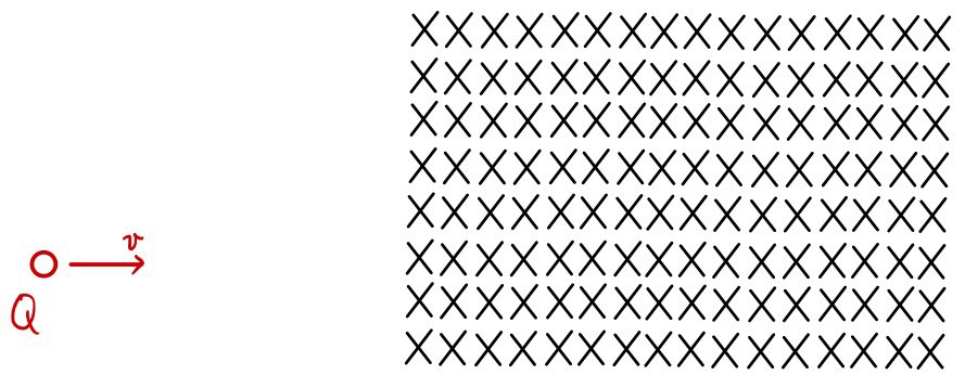
At entry, \(\mathbf v\) points right and \(\mathbf B\) points into the page. Therefore \(\mathbf v\times\mathbf B\) points upward. Because the illustrated charge is positive, the magnetic force also points upward.

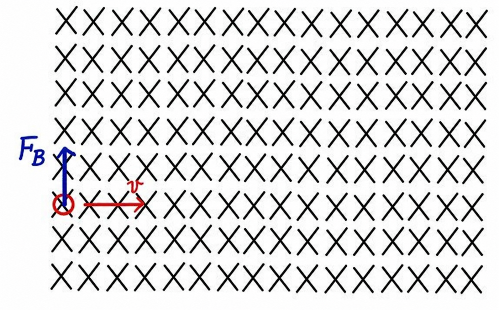
As the velocity turns, the force turns with it and remains perpendicular to the instantaneous velocity.

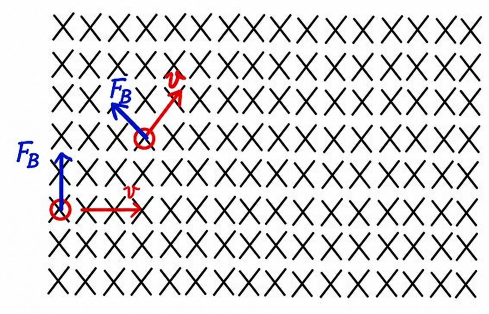
For a nonzero charge in a uniform \(\mathbf B\), with \(\mathbf E=0\) and no other forces acting, a nonzero velocity component perpendicular to \(\mathbf B\) makes the magnetic force supply the centripetal acceleration. The motion is circular when the parallel component is zero. When both perpendicular and parallel components are nonzero, the unaffected parallel component combines with the circular motion to produce a helix. A negative charge curves in the opposite sense from the positive charge shown in the diagrams.

Why the magnetic force does no work

For the magnetic part of the Lorentz force,

\[ \begin{aligned} dW_B &=\mathbf F_B\cdot d\mathbf r \\ &=q\left(\mathbf v\times\mathbf B\right)\cdot\mathbf v\,dt \\ &=0. \end{aligned} \]

The scalar triple product is zero because \(\mathbf v\times\mathbf B\) is perpendicular to \(\mathbf v\). A magnetic field can therefore change a particle’s direction, but the magnetic force alone cannot change its kinetic energy. The electric part \(q\mathbf E\) can do work.

Current is a scalar; current density is a vector

Conventional current through an oriented cross-section is the signed rate at which charge crosses it:

\[ \boxed{ I=\frac{dq}{dt} }. \]

Its SI unit is the ampere, with \(1\ \mathrm A=1\ \mathrm C/\mathrm s\). Once the positive direction of the wire is chosen, \(I\) is a signed scalar, not a vector. A negative value means that the conventional current is opposite the chosen orientation.

For charge confined to a thin line, let \(\lambda\) be the linear charge density and let \(v_{\parallel}\) be the signed carrier velocity along the chosen tangent. Then

\[ \boxed{ I=\lambda v_{\parallel} }. \]

The surface and volume descriptions use vector current densities:

\[ \boxed{ \mathbf K=\sigma\mathbf v_{\parallel} }, \qquad \boxed{ \mathbf J=\rho\mathbf v }. \]

Here \(\sigma\) is surface charge density, \(\mathbf v_{\parallel}\) is the velocity component tangent to the surface, and \(\mathbf K\) is surface current density with units \(\mathrm{A/m}\). Likewise, \(\rho\) is volume charge density and \(\mathbf J\) is volume current density with units \(\mathrm{A/m^2}\). The vector \(\mathbf J\) describes both how much conventional current flows locally and the direction in which positive charge would flow.

The current through an oriented surface \(S\) is related to \(\mathbf J\) by

\[ I=\int_S \mathbf J\cdot d\mathbf a. \]

Thus \(\mathbf J\) is current per unit area normal to the flow; it is not current per unit volume.

Magnetic force on continuous currents

Starting from the force on one moving charge,

\[ d\mathbf F=dq\,\mathbf v\times\mathbf B, \]

we can sum the force over a continuous distribution. In this section, \(\mathbf B\) denotes the specified applied or external magnetic field; a current distribution’s force due to its own generally singular field requires a separate self-force treatment. The correct measure depends on the dimension of the distribution.

For a thin wire, choose an orientation for the directed line element \(d\boldsymbol{\ell}=\hat{\mathbf t}\,d\ell\), and take the scalar current \(I\) as positive or negative relative to that orientation. Then

\[ \boxed{ \mathbf F =\int_C I\,d\boldsymbol{\ell}\times\mathbf B }. \]

For a surface current density \(\mathbf K\),

\[ \boxed{ \mathbf F =\int_S \left(\mathbf K\times\mathbf B\right)\,da }. \]

For a volume current density \(\mathbf J\),

\[ \boxed{ \mathbf F =\int_V \left(\mathbf J\times\mathbf B\right)\,d\tau }. \]

These are line, surface, and volume integrals respectively. The elements \(d\boldsymbol{\ell}\), \(da\), and \(d\tau\) are not interchangeable. The fields may vary with position, so each integrand is evaluated locally over its stated domain.

Charge conservation and steady current

Charge conservation is expressed locally by the continuity equation:

\[ \boxed{ \frac{\partial\rho}{\partial t}+\nabla\cdot\mathbf J=0 }. \]

It says that if charge density inside a small region changes, there must be a corresponding net current through the region’s boundary.

In a steady state,

\[ \frac{\partial\rho}{\partial t}=0, \]

so the continuity equation gives

\[ \boxed{ \nabla\cdot\mathbf J=0 }. \]

This is the precise local statement that steady current does not pile charge up inside the conductor. Magnetostatics additionally takes the macroscopic current distribution itself to be time independent, \(\partial\mathbf J/\partial t=0\). A claim that one scalar current is constant should not, by itself, be treated as equivalent to both of these field conditions.

Source and editorial note

This edition is based on the original Korean article identified in the page metadata. It preserves the original progression from magnetostatics and the Lorentz force to current distributions and charge continuity, as well as all three trajectory diagrams; the two diagrams that contained Korean magnetic-force labels are localized with the exact label \(F_B\). For scientific accuracy and accessibility, it replaces raster equations with native TeX and corrects the steady-current assumptions, charge-sign convention, scalar-versus-vector current distinction, definitions of \(\mathbf K\) and \(\mathbf J\), differential measures in the force integrals, and the relation between the continuity equation and steady state.