The Biot–Savart Law

Previously, we studied the force on a moving charge in a magnetic field. A moving charge is not, by itself, an electric current: current is the rate at which charge crosses a surface. In a wire, however, the organized motion of many charge carriers does produce a current.

A steady current creates a magnetic field that is steady in time but generally varies from point to point. So how large is that field, and how does it depend on the current and geometry? The Biot–Savart law gives us the answer.

The Biot–Savart law

Consider a directed line element $d\boldsymbol{\ell}'$ at source position $\mathbf r'$, carrying a steady current $I$. Let the observation point be $\mathbf r$, and define

$$ \boldsymbol{\eta}=\mathbf r-\mathbf r', \qquad \eta=\lvert\boldsymbol{\eta}\rvert, \qquad \hat{\boldsymbol{\eta}}=\frac{\boldsymbol{\eta}}{\eta}. $$

The element contributes

$$ d\mathbf B(\mathbf r) =\frac{\mu_0 I}{4\pi} \frac{d\boldsymbol{\ell}'\times\hat{\boldsymbol{\eta}}}{\eta^2} =\frac{\mu_0 I}{4\pi} \frac{d\boldsymbol{\ell}'\times\boldsymbol{\eta}}{\eta^3}. $$

Adding the contributions from the entire wire gives the Biot–Savart law:

$$ \boxed{ \mathbf B(\mathbf r) =\frac{\mu_0 I}{4\pi} \int_C\frac{d\boldsymbol{\ell}'\times\hat{\boldsymbol{\eta}}}{\eta^2} } $$

Here $\mu_0$ is the permeability of vacuum. In the current SI it is experimentally determined; its familiar textbook value is approximately

$$ \mu_0\approx4\pi\times10^{-7}\ \mathrm{N/A^2}, \qquad 1\ \mathrm T=1\ \mathrm{N/(A\,m)}. $$

The cross product fixes the field direction by the right-hand rule. Its magnitude contains $\sin\alpha$, where $\alpha$ is the angle between $d\boldsymbol{\ell}'$ and $\boldsymbol{\eta}$.

Magnetic field of a finite straight wire

Let point $P$ be a perpendicular distance $s$ from a straight wire carrying current $I$. The first sketch establishes the geometry.

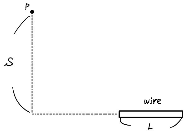
For an element at coordinate $\ell$, define signed $\theta$ at $P$ from the downward perpendicular toward the source direction $-\boldsymbol{\eta}$ shown in the sketch. Then

$$ \ell=s\tan\theta, \qquad \eta=s\sec\theta, \qquad d\ell=s\sec^2\theta\,d\theta. $$

For current toward increasing $\ell$, the directed angle between $d\boldsymbol{\ell}'$ and $\boldsymbol{\eta}$ is $\alpha=\pi/2+\theta$. Therefore $\sin\alpha=\sin(\pi/2+\theta)=\cos\theta$, so the scalar integrand and final magnitude below are unchanged. Every contribution points along the same normal direction $\hat{\mathbf n}$, as determined by the right-hand rule.

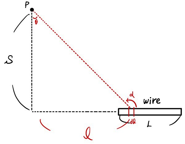
Therefore,

$$ \begin{aligned} \mathbf B &=\frac{\mu_0 I}{4\pi}\hat{\mathbf n} \int_{\theta_1}^{\theta_2} \frac{d\ell\cos\theta}{\eta^2} \\ &=\frac{\mu_0 I}{4\pi s}\hat{\mathbf n} \int_{\theta_1}^{\theta_2}\cos\theta\,d\theta \\ &=\boxed{ \frac{\mu_0 I}{4\pi s} \left(\sin\theta_2-\sin\theta_1\right)\hat{\mathbf n} }. \end{aligned} $$

The endpoint angles $\theta_1$ and $\theta_2$ are signed according to the convention in the sketch. This explicit convention is important; otherwise a memorized plus or minus sign can be misleading.

Infinite straight wire

For a wire extending from $-\infty$ to $+\infty$,

$$ \theta_1=-\frac{\pi}{2}, \qquad \theta_2=\frac{\pi}{2}. $$

The result becomes

$$ \boxed{ \mathbf B=\frac{\mu_0 I}{2\pi s}\hat{\mathbf n} }. $$

So the magnetic field of an infinitely long straight wire is proportional to $I$ and decreases as $1/s$, not as $1/s^2$. This is the familiar high-school result, now derived rather than simply quoted. If one writes $B=kI/s$ in SI units, then $k=\mu_0/(2\pi)$.

Magnetic field on the axis of a circular current loop

Now consider a circular loop of radius $R$ carrying current $I$. We want the field at a point on its symmetry axis, a distance $z$ from the center.

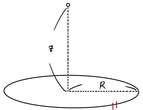
For every point on the loop,

$$ \eta=\sqrt{R^2+z^2}. $$

The current element $d\boldsymbol{\ell}'$ is perpendicular to $\boldsymbol{\eta}$, so

$$ dB=\frac{\mu_0 I}{4\pi}\frac{d\ell}{R^2+z^2}. $$

The next sketch shows the directions. Define positive $I$ to follow the direction of $d\boldsymbol{\ell}'$ shown there. For that orientation, the right-hand rule makes the surviving axial component point along $+\hat{\mathbf z}$. By azimuthal symmetry, the components perpendicular to the axis cancel in pairs, while the axial components add. Reversing the current reverses the magnetic field.

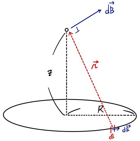
If $\beta$ is the angle between $d\mathbf B$ and the axis, the geometry gives

$$ \cos\beta=\frac{R}{\sqrt{R^2+z^2}}. $$

Thus

$$ \begin{aligned} \mathbf B(z) &=\hat{\mathbf z}\int dB\cos\beta \\ &=\hat{\mathbf z}\frac{\mu_0 I}{4\pi} \frac{R}{\left(R^2+z^2\right)^{3/2}} \oint d\ell \\ &=\boxed{ \frac{\mu_0 I R^2}{2\left(R^2+z^2\right)^{3/2}} \hat{\mathbf z} }. \end{aligned} $$

At the center of the loop, $z=0$, this reduces to

$$ \mathbf B(0)=\frac{\mu_0 I}{2R}\hat{\mathbf z}. $$

Nice! With one law and some geometry, we have obtained the field of a finite straight wire, its infinite-wire limit, and the on-axis field of a circular loop.

---

Source note: This English edition follows the examples and order of the original Korean post. It replaces legacy formula screenshots with accessible native mathematics and explicitly corrects the original wording that treated a moving charge as current and a spatially varying steady field as “constant.” The notation and angle conventions have also been made explicit.