Ampère's Law

In electrostatics, Gauss’s law relates electric flux through a closed surface to enclosed charge. In magnetostatics, Ampère’s law relates the circulation of the magnetic field around a closed curve to the steady current passing through a surface bounded by that curve.

That distinction—surface flux versus line circulation—is essential. We will first derive the magnetostatic result, then add Maxwell’s displacement-current term for time-dependent fields.

Magnetic field around a long straight wire

Consider an infinitely long wire on the $z$-axis carrying a steady current $I$ in the $+z$ direction, out of the page. Let $\rho$ be the perpendicular distance from the wire.

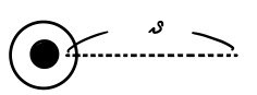
The Biot–Savart law gives

$$ \boxed{ \mathbf B(\rho)=\frac{\mu_0 I}{2\pi\rho}\,\hat{\boldsymbol\phi} }. $$

The right-hand rule fixes the azimuthal direction $\hat{\boldsymbol\phi}$.

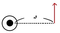
Now choose a counterclockwise circular contour $C$ of radius $R$ centered on the wire. The field is tangent to the contour and has constant magnitude on it.

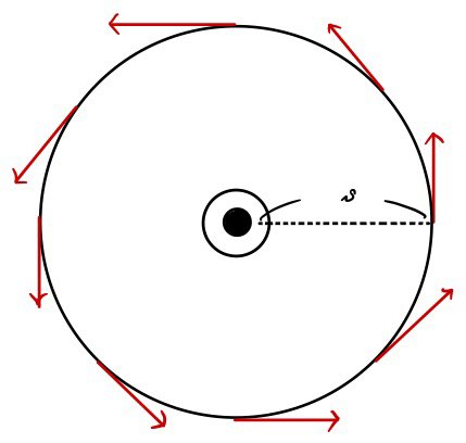
Therefore,

$$ \begin{aligned} \oint_C \mathbf B\cdot d\boldsymbol\ell &=\int_0^{2\pi} \left(\frac{\mu_0 I}{2\pi R}\right)R\,d\phi \\ &=\mu_0 I. \end{aligned} $$

The original formula image described this step by noting that $\mathbf B$ and $d\boldsymbol\ell$ point in the same direction on this centered circle. Written as a dot product, the statement is precise and accessible.

The contour need not be centered on the wire

Move the wire away from the center of the same circular contour while keeping it inside.

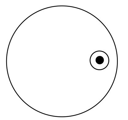
The straight-wire field still has magnitude $\mu_0 I/(2\pi\rho)$, but now the local distance $\rho$ varies around the circle. The field is also not generally tangent to the contour, so we must integrate the projection $\mathbf B\cdot d\boldsymbol\ell$ rather than multiply a single field magnitude by the circumference.

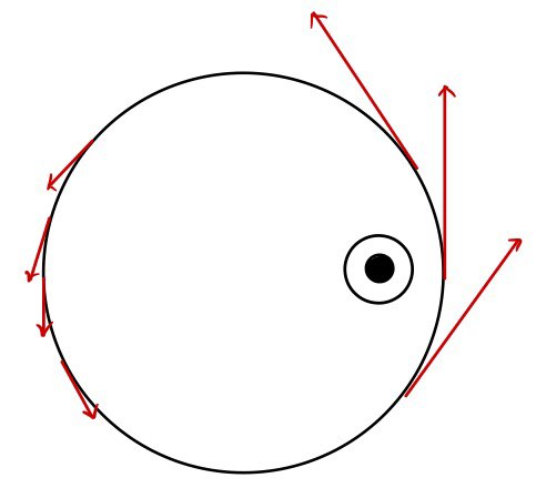
For an explicit check, place the wire at $(a,0)$ and parameterize a counterclockwise circle of radius $R$ centered at the origin:

$$ \mathbf r(\phi)=(R\cos\phi,R\sin\phi), \qquad d\boldsymbol\ell=(-R\sin\phi,R\cos\phi)\,d\phi. $$

The squared distance from the wire is

$$ \rho^2=R^2+a^2-2aR\cos\phi, $$

and the field on the contour is

$$ \mathbf B =\frac{\mu_0 I}{2\pi\rho^2} (-R\sin\phi,\,R\cos\phi-a). $$

Thus,

$$ \mathbf B\cdot d\boldsymbol\ell =\frac{\mu_0 I}{2\pi} \frac{R(R-a\cos\phi)}{R^2+a^2-2aR\cos\phi}\,d\phi. $$

Integrating from $0$ to $2\pi$ gives $\mu_0 I$ when $|a| < R$. More generally,

$$ \oint_C \mathbf B\cdot d\boldsymbol\ell =\mu_0 I\,n(C,\text{wire}), $$

where $n(C,\text{wire})$ is the signed winding number. It is $1$ for a simple positively oriented loop enclosing the wire, $0$ when the wire is outside, and the ideal filament model is singular if the wire lies on $C$.

This exact projection calculation replaces the tempting but unreliable idea that a stronger field over a shorter part of the path simply cancels a weaker field over a longer part.

General magnetostatic Ampère’s law

Let $C=\partial S$ be a closed contour bounding an oriented surface $S$. The right-hand rule links the positive direction around $C$ to the surface normal. For steady currents,

$$ \boxed{ \oint_C \mathbf B\cdot d\boldsymbol\ell =\mu_0 I_{\mathrm{enc}} }, \qquad I_{\mathrm{enc}}=\iint_S \mathbf J\cdot d\mathbf a. $$

$I_{\mathrm{enc}}$ is signed: currents piercing $S$ in opposite directions contribute with opposite signs, and multiple currents add algebraically. Any closed contour can be called an Amperian loop; in practice, we choose one that exploits the symmetry of the field.

For comparison, Gauss’s law for the electric field is a closed-surface flux law:

$$ \oiint_S \mathbf E\cdot d\mathbf a =\frac{Q_{\mathrm{enc}}}{\varepsilon_0}. $$

The analogy is useful, but the geometric objects differ: Ampère’s law uses circulation around a closed curve, whereas Gauss’s law uses flux through a closed surface.

Maxwell’s time-dependent correction

The magnetostatic equation is incomplete when the electric flux changes with time. For a fixed contour $C$ and an oriented spanning surface $S$, the Maxwell–Ampère law is

$$ \boxed{ \oint_C \mathbf B\cdot d\boldsymbol\ell =\mu_0\iint_S \mathbf J\cdot d\mathbf a +\mu_0\varepsilon_0\frac{d}{dt} \iint_S \mathbf E\cdot d\mathbf a }. $$

Equivalently,

$$ \boxed{ \boldsymbol\nabla\times\mathbf B =\mu_0\mathbf J +\mu_0\varepsilon_0\frac{\partial\mathbf E}{\partial t} }. $$

The displacement-current term involving the changing electric flux is what makes the integral law consistent when different surfaces share the same boundary. In the magnetostatic limit, $\partial\mathbf E/\partial t=0$, and the earlier form is recovered.

Stokes’ theorem and the curl of the magnetic field

For a sufficiently smooth field on the oriented surface $S$, Stokes’ theorem gives

$$ \oint_C \mathbf B\cdot d\boldsymbol\ell =\iint_S (\boldsymbol\nabla\times\mathbf B)\cdot d\mathbf a. $$

Combining this with the steady-current law,

$$ \iint_S (\boldsymbol\nabla\times\mathbf B)\cdot d\mathbf a =\mu_0\iint_S \mathbf J\cdot d\mathbf a. $$

Because this holds for every sufficiently small suitable surface in magnetostatics,

$$ \boxed{ \boldsymbol\nabla\times\mathbf B=\mu_0\mathbf J }. $$

This is the magnetostatic limit, not the complete time-dependent Maxwell equation displayed above.

Why the divergence of the magnetic field is zero

For a smooth, localized, steady current distribution, the Biot–Savart law can be written

$$ \mathbf B(\mathbf r) =\frac{\mu_0}{4\pi} \int \mathbf J(\mathbf r')\times \frac{\mathbf R}{R^3} \,d^3r', $$

where

$$ \mathbf R=\mathbf r-\mathbf r', \qquad R=\lvert\mathbf R\rvert, \qquad d^3r'=dx'\,dy'\,dz'. $$

Here $\mathbf r$ is the observation coordinate and $\mathbf r'$ is the independent source coordinate. Define

$$ \mathbf F(\mathbf R)=\frac{\mathbf R}{R^3} =-\boldsymbol\nabla_{\mathbf r}\!\left(\frac{1}{R}\right). $$

Assuming the regularity needed to differentiate under the integral, we obtain

$$ \begin{aligned} \boldsymbol\nabla_{\mathbf r}\cdot\mathbf B(\mathbf r) &=\frac{\mu_0}{4\pi} \int \boldsymbol\nabla_{\mathbf r}\cdot \left[\mathbf J(\mathbf r')\times\mathbf F(\mathbf R)\right]d^3r' \\ &=\frac{\mu_0}{4\pi} \int\!\left\{ \mathbf F\cdot \left[\boldsymbol\nabla_{\mathbf r}\times\mathbf J(\mathbf r')\right] -\mathbf J(\mathbf r')\cdot \left[\boldsymbol\nabla_{\mathbf r}\times\mathbf F\right] \right\}d^3r'. \end{aligned} $$

The two terms vanish for different reasons. First,

$$ \boldsymbol\nabla_{\mathbf r}\times\mathbf J(\mathbf r')=\mathbf 0 $$

because $\mathbf r$ and $\mathbf r'$ are independent variables. This does not say that the physical source-coordinate curl $\boldsymbol\nabla_{\mathbf r'}\times\mathbf J(\mathbf r')$ must vanish. Second,

$$ \boldsymbol\nabla_{\mathbf r}\times\mathbf F=\mathbf 0 $$

because $\mathbf F$ is a gradient field. The statement is immediate away from $\mathbf R=\mathbf 0$ and remains valid in the distributional treatment of the full integral. Therefore,

$$ \boxed{ \boldsymbol\nabla\cdot\mathbf B=0 }. $$

Equivalently, the net magnetic flux through every closed surface is zero:

$$ \oiint_S \mathbf B\cdot d\mathbf a=0. $$

This is Gauss’s law for magnetism, one of Maxwell’s equations beyond the magnetostatic derivation used here. In standard classical electromagnetism there is no magnetic-charge density term, so magnetic field lines do not begin or end at isolated magnetic charges. No isolated magnetic monopole has been experimentally confirmed; if magnetic charge were discovered, the field equations would need a corresponding source term.

---

Source and correction note: This English edition follows the original progression from a straight wire through Ampère’s integral and differential laws to $\boldsymbol\nabla\cdot\mathbf B=0$. The five source diagrams remain in their restored order. Ten legacy formula images—including the Korean parenthetical in the centered-loop calculation and the Korean labels in the Stokes and divergence steps—are replaced with accessible native mathematics and English explanation. Scientific corrections are explicit: the off-center calculation uses the local tangential projection, the magnetostatic scope is separated from Maxwell’s time-dependent law, primed and unprimed derivatives are distinguished, and the monopole conclusion is stated as a classical field law and observational status rather than a proof of nonexistence.