Ampère's Law: Three Symmetry Examples

Ampère’s law is most useful when symmetry tells us the direction of the magnetic field and makes its magnitude constant along a carefully chosen path. The law is always valid for steady currents, but it does not automatically make every geometry easy.

The source first compares Gauss’s law with Ampère’s law. Gauss’s law relates the electric flux through a closed surface $S$ to the enclosed charge $Q_{\mathrm{in}}$:

$$ \oint_S \mathbf E\cdot d\mathbf a =\frac{Q_{\mathrm{in}}}{\varepsilon_0}, \qquad \nabla\cdot\mathbf E=\frac{\rho}{\varepsilon_0}. $$

In magnetostatics, Ampère’s law gives the corresponding circulation and differential relations

$$ \oint_C \mathbf B\cdot d\boldsymbol\ell =\mu_0 I_{\mathrm{in}}, \qquad \nabla\times\mathbf B=\mu_0\mathbf J. $$

Here $C=\partial S$ is oriented with its spanning surface by the right-hand rule, and $I_{\mathrm{in}}$ (also written $I_{\mathrm{enc}}$ below) is the signed current through that surface:

$$ I_{\mathrm{enc}}=\iint_S \mathbf J\cdot d\mathbf a. $$

The sign of $I_{\mathrm{enc}}$ depends on the chosen surface normal. Reversing the contour reverses both the line integral and the positive normal, so the physical result is unchanged. The comparison is structural: Gauss’s law uses electric flux through a closed surface and divergence, whereas magnetostatic Ampère’s law uses magnetic circulation around a closed contour and curl.

This lesson applies Ampère’s law to three idealized examples.

1. Infinite straight wire

Place an infinitely long, thin wire on the $z$-axis and let it carry a steady current $I$ in the $+z$ direction. Write $s$ for the perpendicular distance from the wire.

Cylindrical symmetry gives two crucial facts:

1. $\mathbf B$ points in the azimuthal direction $\hat{\boldsymbol\phi}$, fixed by the right-hand rule.
2. Its magnitude depends only on $s$, so it is constant on a circle centered on the wire.

Choose a counterclockwise circular Amperian loop of radius $s$ as viewed from $+z$. Along that loop, $\mathbf B$ is parallel to $d\boldsymbol\ell$, and the loop encloses current $I$. Therefore,

$$ \begin{aligned} \oint_C \mathbf B\cdot d\boldsymbol\ell &=B(s)\oint_C d\ell \\ &=B(s)(2\pi s) =\mu_0 I. \end{aligned} $$

Hence

$$ \boxed{ \mathbf B(s)=\frac{\mu_0 I}{2\pi s}\,\hat{\boldsymbol\phi} }. $$

The shortcut $B(2\pi s)$ is justified by symmetry; it is not a generic consequence of Ampère’s law.

2. Infinite surface-current sheet

Now consider the plane $z=0$ carrying a uniform surface current density

$$ \mathbf K=K\,\hat{\mathbf x}, $$

where $K$ has units of amperes per metre.

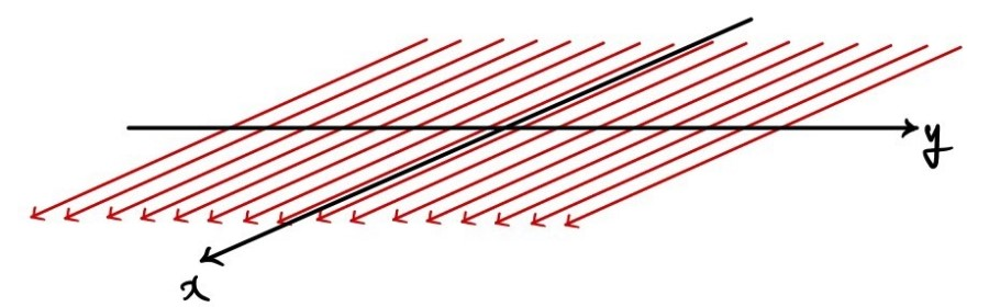
Translational symmetry in $x$ and $y$ means that the field cannot depend on position within either half-space. The right-hand rule and reflection symmetry show that the field is parallel to the sheet, perpendicular to $\mathbf K$, and reverses direction across the sheet. Thus we may write

$$ \mathbf B_{z>0}=-B_0\,\hat{\mathbf y}, \qquad \mathbf B_{z<0}=+B_0\,\hat{\mathbf y}. $$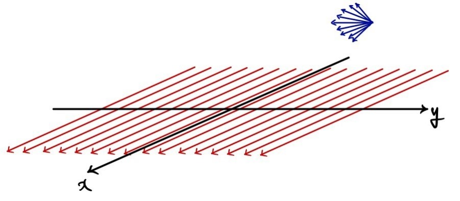

Choose a rectangular Amperian loop in a plane perpendicular to the sheet current. Let each long side have length $L$ and run parallel to the $y$-axis, with one long side above the sheet and the other below it. Orient the loop so its surface normal is $+\hat{\mathbf x}$.

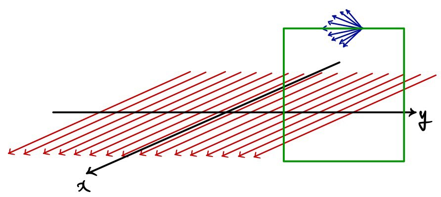
The two short sides are perpendicular to $\mathbf B$ and contribute zero. With the chosen orientation, $\mathbf B$ is parallel to $d\boldsymbol\ell$ on both long sides, so

$$ \oint_C \mathbf B\cdot d\boldsymbol\ell=2B_0L. $$

The sheet current piercing the spanning surface is

$$ I_{\mathrm{enc}}=KL. $$

Ampère’s law therefore gives

$$ 2B_0L=\mu_0KL, \qquad B_0=\frac{\mu_0K}{2}. $$

The complete vector result is

$$ \boxed{ \mathbf B(z)= \begin{cases} -\dfrac{\mu_0K}{2}\,\hat{\mathbf y}, & z>0,\\[6pt] +\dfrac{\mu_0K}{2}\,\hat{\mathbf y}, & z<0. \end{cases} } $$

Equivalently, if $\hat{\mathbf n}=\hat{\mathbf z}$ points from the lower side to the upper side, the jump condition is

$$ \hat{\mathbf n}\times (\mathbf B_{\mathrm{above}}-\mathbf B_{\mathrm{below}}) =\mu_0\mathbf K. $$

3. Ideal infinite solenoid

Model a tightly wound, infinitely long solenoid of radius $R$ as a cylindrical surface current. Let the axis be the $z$-axis, let $n$ be the number of turns per unit length, and let each turn carry current $I$. The equivalent surface-current magnitude is $K=nI$.

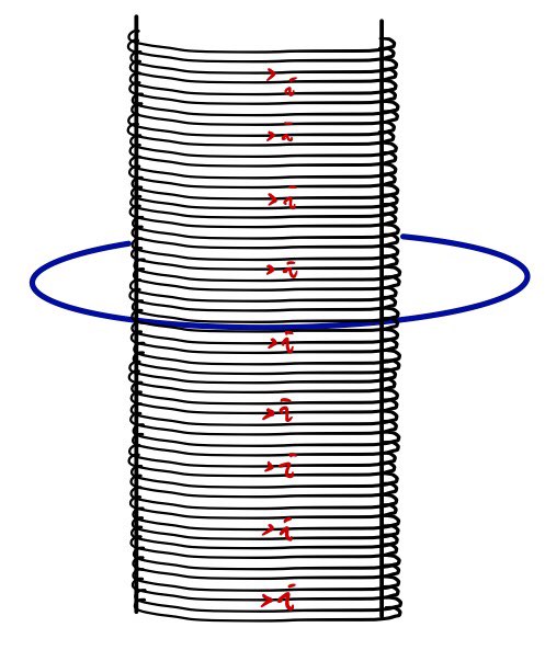
The blue circular path in the source diagram is useful for one warning. Because an ideal solenoid’s field is axial while $d\boldsymbol\ell$ on that circle is azimuthal,

$$ \oint_C \mathbf B\cdot d\boldsymbol\ell=0 $$

whether or not the axial field is zero. A zero circulation around that particular path does not, by itself, prove that the outside axial field vanishes.

For the ideal infinite-solenoid model, translational and rotational symmetry fix the field’s axial form and its independence from $z$ and azimuth. Rectangular Amperian-loop comparisons within each current-free region then establish that the axial field is constant with radius there, so we may write

$$\mathbf B=\begin{cases} B_{\mathrm{in}}\,\hat{\mathbf z}, & s\lt R,\\[6pt] B_{\mathrm{out}}\,\hat{\mathbf z}, & s\gt R. \end{cases}$$

with the sign of $\hat{\mathbf z}$ chosen by the right-hand rule around the winding.

A rectangular loop whose two long sides are parallel to the $z$-axis gives the useful comparison. If both long sides lie outside, no surface current crosses the loop, so $B_{\mathrm{out}}$ is the same at every exterior radius. The physical boundary condition $\mathbf B\to\mathbf 0$ far from the ideal solenoid then fixes

$$ \boxed{\mathbf B_{\mathrm{out}}=\mathbf 0}. $$

This conclusion uses symmetry and the boundary condition at infinity, not Ampère’s law alone.

Now place one long side of the rectangular loop inside the solenoid and the other outside.

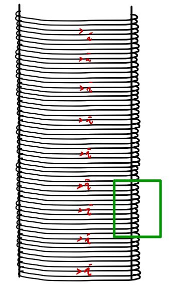
Let each long side have length $L$. The short sides are perpendicular to the axial field, and the outside long side contributes zero. The spanning surface cuts $nL$ turns, each carrying current $I$, so the magnitude of the enclosed current is

$$ I_{\mathrm{enc}}=(nL)I. $$

With the contour orientation chosen to make the enclosed current positive,

$$ \begin{aligned} \oint_C\mathbf B\cdot d\boldsymbol\ell &=B_{\mathrm{in}}L \\ &=\mu_0(nL)I. \end{aligned} $$

Therefore,

$$ \boxed{ \mathbf B_{\mathrm{in}}=\mu_0nI\,\hat{\mathbf z} }, $$

where the right-hand rule determines whether the field is $+\hat{\mathbf z}$ or $-\hat{\mathbf z}$ for the actual winding direction.

A real finite solenoid has a nonzero fringe field outside. Near the center of a solenoid whose length is much greater than its radius, $B\approx\mu_0nI$ is a useful approximation; it is exact only in the ideal infinite model used above.

What the three examples teach

• Straight wire: cylindrical symmetry makes $B$ constant and tangent on a circular path.
• Current sheet: planar symmetry makes the two long sides of a rectangular path contribute equally.
• Ideal solenoid: symmetry establishes the field’s form, while a rectangular loop gives the jump across the surface current; the outside value also requires a boundary condition.

The recurring method is to establish the field direction and spatial dependence first, then choose a contour on which the line integral simplifies.

---

Source and correction note: This English edition follows the three-example sequence and preserves the five source-bound diagrams from the original Korean source recorded in the page metadata. The six small formula images are replaced with accessible native mathematics and English explanation, including the source’s opening Gauss-law and Ampère-law integral/differential comparison. The standard straight-wire and ideal-solenoid results were cross-checked against OpenStax University Physics Volume 2, §12.5 and §12.6. A scientific correction is made explicit: zero circulation around the original exterior circular path does not prove that an axial exterior field is zero; the ideal-solenoid result also uses symmetry and the boundary condition at infinity.