Magnetic Vector Potential: What Does B = Curl A Mean?

In electrostatics, the electric field is curl-free:

$$ \nabla\times\mathbf E=\mathbf 0. $$

On a suitable domain, that lets us introduce a scalar potential $V$ and write

$$ \mathbf E=-\nabla V. $$

Magnetostatics starts from a different Maxwell equation:

$$ \nabla\cdot\mathbf B=0. $$

Because the magnetic field has zero divergence, it can be represented locally—and globally when the domain has the required topology—as the curl of a vector field:

$$ \boxed{\mathbf B=\nabla\times\mathbf A}. $$

The field $\mathbf A$ is the magnetic vector potential. But what does that equation actually mean?

A pinwheel picture for curl

My original way into curl was to imagine placing a tiny pinwheel in a vector field. The first source sketch is the pinwheel itself.

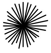
If the surrounding arrows tend to drive one side one way and the other side the opposite way, the pinwheel suggests a local sense of rotation.

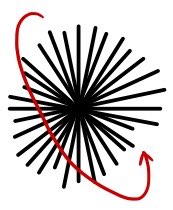
The direction of the curl is perpendicular to the plane of that rotation, with its sign set by the right-hand rule. In the source picture, that direction is labeled $\mathbf B$.

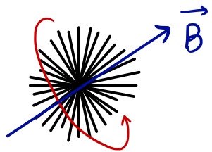
So the useful part of the analogy is this:

$$ \mathbf B(\mathbf r)=\nabla\times\mathbf A(\mathbf r) $$

means that $\mathbf B$ records the local circulation density of $\mathbf A$, including its axis and orientation.

The picture has limits. $\mathbf A$ is not a wind, force, or velocity field, and an actual pinwheel placed in space would not literally spin because of $\mathbf A$. Curl is a spatial derivative of a field, not the angular speed of a test object. Likewise, divergence does not say that an object must fly away or remain fixed. Those statements in the historical intuition were too literal.

There is one special mathematical connection worth keeping separate: for a rigid-body velocity field, the local angular velocity is one-half of the curl. That fact does not turn the magnetic vector potential into a mechanical velocity.

From Ampère’s law to a Poisson equation for A

For steady currents, Ampère’s law in differential form is

$$ \nabla\times\mathbf B=\mu_0\mathbf J. $$

Substituting $\mathbf B=\nabla\times\mathbf A$ gives

$$ \nabla\times(\nabla\times\mathbf A)=\mu_0\mathbf J. $$

The restored source equation records that substitution and then uses the vector identity

$$ \nabla\times(\nabla\times\mathbf A) =\nabla(\nabla\cdot\mathbf A)-\nabla^2\mathbf A. $$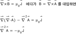

The last step in the source image silently chooses the Coulomb gauge,

$$ \nabla\cdot\mathbf A=0. $$

With that gauge condition,

$$ \boxed{\nabla^2\mathbf A=-\mu_0\mathbf J}. $$

This is a vector Poisson equation. It parallels the electrostatic equation

$$ \nabla^2V=-\frac{\rho}{\varepsilon_0}. $$

The restored comparison image places the two Poisson equations and their Green-function solutions side by side. Its short Korean label says that the magnetic result is obtained “in the same context as electrostatics.”

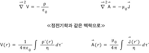
For steady, localized currents and the boundary condition $\mathbf A\to\mathbf 0$ at infinity, the Coulomb-gauge solution is

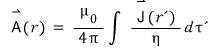
$$ \boxed{ \mathbf A(\mathbf r) =\frac{\mu_0}{4\pi} \int \frac{\mathbf J(\mathbf r')}{\lvert\mathbf r-\mathbf r'\rvert} \,d\tau' }. $$

Writing

$$ \eta=\lvert\mathbf r-\mathbf r'\rvert, $$

the same expression appears in the next source equation.

Reading the current integral

The integration variable $\mathbf r'$ labels a source point, while $\mathbf r$ is the observation point. Each small source volume $d\tau'$ contributes

$$ d\mathbf A(\mathbf r) =\frac{\mu_0}{4\pi} \frac{\mathbf J(\mathbf r')}{\eta} \,d\tau'. $$

The source drawing pictures three pieces of a current distribution at three different distances from one observation point.

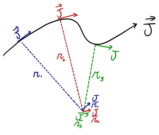
For equal current-density magnitudes and equal source-volume elements, the $1/\eta$ factor makes a nearer contribution larger than a farther one:

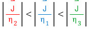
This weighting should not be read as saying that $\mathbf A$ is simply “$1/\eta$ times smaller than $\mathbf J$.” The two quantities have different physical dimensions, and the integral combines contributions from the entire current distribution. Each individual integrand contribution is parallel to its own $\mathbf J(\mathbf r')$, but the direction of the total $\mathbf A$ depends on all source points and on the chosen gauge.

Taking the curl of this $\mathbf A$ recovers the magnetic field. For a steady localized current, the result can be written in the Biot–Savart form

$$ \mathbf B(\mathbf r) =\frac{\mu_0}{4\pi} \int \frac{\mathbf J(\mathbf r')\times(\mathbf r-\mathbf r')} {\lvert\mathbf r-\mathbf r'\rvert^3} \,d\tau'. $$

The final source sketch combines a current element, its separation from the observation point, the pinwheel picture, and the direction of $\mathbf B$.

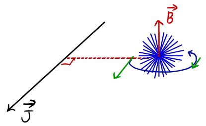
The sketch is a reminder of the original intuition, but the equations now tell us precisely what is happening: the current distribution determines $\mathbf A$ through the Green-function integral, and the spatial curl of $\mathbf A$ determines $\mathbf B$.

A is not unique

Different vector potentials can describe the same magnetic field. If $\chi$ is a sufficiently smooth scalar field, then

$$ \mathbf A' = \mathbf A+\nabla\chi $$

gives

$$ \nabla\times\mathbf A' =\nabla\times\mathbf A =\mathbf B, $$

because the curl of a gradient is zero. This is gauge freedom. The Coulomb gauge used above is a convenient choice that turns Ampère’s law into a Poisson equation; it is not an extra magnetic field law.

What to keep from the intuition

• $\mathbf B=\nabla\times\mathbf A$ says that the magnetic field is the local curl of the vector potential.
• The pinwheel sketches visualize orientation and circulation, not literal force, translation, or angular speed.
• In Coulomb gauge, a steady localized current obeys $\nabla^2\mathbf A=-\mu_0\mathbf J$.
• With $\mathbf A\to\mathbf 0$ at infinity, the solution weights each source-current contribution by $1/\lvert\mathbf r-\mathbf r'\rvert$.
• Only $\mathbf B$ is fixed by the curl relation; $\mathbf A$ retains gauge freedom.

One notation reminder from the source: bold symbols such as $\mathbf J$ and $\mathbf A$ denote vectors, while their magnitudes are written $\lvert\mathbf J\rvert$ and $\lvert\mathbf A\rvert$.

---

Source and correction note: This English edition follows the original Korean post recorded in the page metadata and preserves its nine source-bound image occurrences in their restored order. Native mathematics and English alt text make the two restored Korean equation images accessible without altering their source pixels. The source’s playful pinwheel idea is retained as a visualization of local circulation, while its literal claims about object motion, angular speed, the direction of the integrated vector potential, and a dimensionless “$1/\eta$ times smaller” comparison are explicitly corrected. The Coulomb-gauge assumption, boundary condition, source-observation separation, and gauge freedom omitted from the historical explanation are stated here.