Gauge Transformations — Coulomb Gauge, Lorenz Gauge, and the d'Alembertian

From now on it’s Chapter 10. Electric potentials and electromagnetic fields.

Up until now we’ve been setting aside the electrostatic state, the steady-current state and so on, and going somewhat more generally since chapters 8 and 9.

But there’s something we haven’t thought about yet — in chapters 8 and 9 we never brought up ’electric potential'.

We only thought about fields (field) like the electric field and the magnetic field.

So in this chapter (chapter), we’re going to think about the potential due to the electric field and the potential due to the magnetic field!!

Um, as we saw before (chapters 2~6), the potential due to the electric field was a scalar, and the potential due to the magnetic field was a vector.

The scalar potential was

The vector potential was

It was like this, right???? But to generalize this a bit more, apparently we need to modify it?

I’ll write that out.

So first let me write down Maxwell’s Equations!!

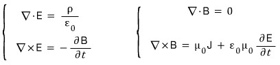
Alright, let’s dive in.

What does it mean to think more more more more than we have so far, you ask —

It means thinking like this.

Originally it was “If E arises, B arises.” We’re turning that into

if there’s E then there’s V, and since B arises, there’s also A.

We’ve already tied E and B together before,

and now I want to tie the scalar potential V and the vector potential A together! Let’s go

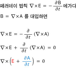
Oh!!!! The red guy is a vector, the blue guy is also a vector!!!! Their sum is also a vector!!!

And the curl of that sum-vector is zero 0, apparently.

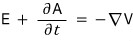
When the curl is 0 — thinking in general-mechanics terms, when the curl of some force F was 0,

Curl is 0 → path-independent → conservative → a scalar potential can be defined.

Ahh, so because that vector

also has curl 0,

apparently we can define a scalar potential!!!

What should we call the scalar Potential???????? C? D? F? GD? Z?

Let’s just call it V.

Okay

Uwaaaaaaa~~~~~~everybody shout it out~~~~~~yeah~~~~

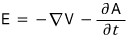
The original formula for the electric potential

we’ve modified this!!!

Like this hehe

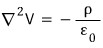
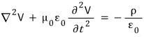
Let’s plug this corrected relation between the electric field and the electric potential into Gauss’s law, equation (i).

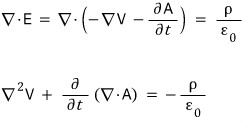
The existing Poisson equation

has been modified

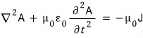
and into the 4th of Maxwell’s equations, too, let’s substitute

.

​

​

​

​

Haa…………… so what am I supposed to do with this lololololololololol ugh whatever!!!!!

Having messed things up this far,

now I’ll get into gauge transformations for real… T_T

But right from the very first line of the first page of the explanation I love it lolololololololololololol

“The above equation, Maxwell’s equations expressed via the potentials, looks unseemly, so you’d want to throw out the formula with the potentials in it.”

​

Kyahahahahaha my mind has been read completely.. lololololololololol

I really do want to throw it out lolololololololol

But we still have to do it…

Let’s jump back for a moment to Chapter 5’s “magnetic vector potential” section.

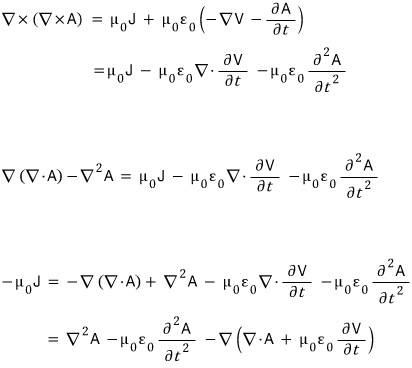
So into Ampère’s law

we plugged the definition in

And then

we said this.

So

​

Now here, when we say

what does this act actually mean………..

Hmm, let’s go to high-school math.​

​

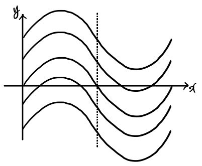
There are 10 functions of the same ‘shape’ (let’s say we did ctrl+c, ctrl+v) — why on earth am I saying this~~​

Those 10 functions are the same shape, so the derivatives of the 10 functions are exactly the same.

​

Why!!!!!

A function, when you put something in, the ‘value’ that comes out is the function value — whereas

a derivative, when you put something in, the ‘value’ that comes out is the ‘slope (differential coefficient)’ at some point.​

​

If I put it more precisely

​

Those 7 functions are each different from one another. But what I wanted to say is that their derivatives are the same.​

​

​

Now, coming back to electromagnetism —

The reason I brought up high-school math just now is,

it’s the same content as electromagnetism, but the math is 1-dimensional and has no meaning attached, so it seemed a bit easier.

It’s just that — yess! — we’ve extended the math story to 3 dimensions, that’s all,

the difference being that y and x have no meaning, but E and V have meaning attached — electric field, electric potential.

Now let me define the potential V’ (V-prime) as

like this

But!!!!!!!!!

with this condition attached (β is a function).

So then, what is the gradient of V-prime over there?

Yes. It’s the same. It’s not some other electric field E’, it’s just E.

Then now let’s really really come back to our original position, the vector potential!!

what this means is the gradient-sense, whereas

​ what this means is rotation.

and here,

let me define A-prime like this

(here too, α must be a function whose curl is zero, right?)

Yes yes yes yes yes yes, so the curl of A’ is also, not B’, but the same as B!?!?!!

Let me add just a bit more about the vector potential.

I’ve been going on and on only about the curl of the vector potential A —

but whether you plug it into Ampère’s law or into the 4th of Maxwell’s equations,

the left-hand side becomes this, so the div of the vector potential A is also something we need to think about.

Earlier, in the steady-current state, the divergence of A was zero~ 0!

Wrong!!!!!!! It’s not that div A is 0 in the steady-current state — it’s that “we set it to 0.”

When we did ∇·A = 0 in Electromagnetism 1, we did it as if it were something obvious,

but it’s not that it’s originally 0 — it’s that in that situation it’s convenient to set it to 0.

“Why can we say ∇·A is ours to choose?”

Let me say it once more — the curl of A’ and the curl of A both produce the same B.

In other words, when we talk about some B, you can call its vector potential A,

or you can call it A’, or A’’, or A’’’, or A’’’’,

and it’s in this sense that in magnetostatics ∇·A = 0 was set.

What should we set ∇·A as~~~~

This — what we set the vector A to be~~~ — is what’s called the Gauge Transformation,

and apparently there are various gauge transformations.

In magnetostatics ∇·A = 0 is convenient; in some other situation ∇·A = ~~~~ is convenient to set,

and in this case-by-case way there are convenient gauge transformations for each situation, and the famous ones, the ones most often used in gauge transformations,

the Coulomb gauge

the Lorenz gauge

are the ones it says we’ll look at.

Alright, we’re finally going into gauge transformations.

Coulomb gauge: setting ∇·A = 0!

Now~ let me bring down those two equations from above.

These ones

Earlier we got this far and then jumped over to the “gauge transformation” stuff out of nowhere,

and now that story is finally connecting back up.

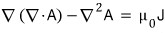
That formula that “seemed useless”

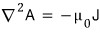
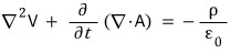
If we take the Coulomb gauge, i.e. set div A = 0, then

(Poisson equation)

(unknown identity)

If we set the Coulomb gauge like that and solve equation 1, the Poisson equation,

(just the electric potential as in electrostatics)

Now, the upside of the Coulomb gauge! :

Calculating V is simple.

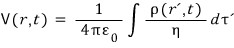
But there’s a downside. “It violates causality.”

Looking at the above equation, if the volume charge density ρ at location r’ changes at time t, at the same time V at location r also changes at time t — that is, simultaneously.

This makes no sense.

What, some kind of remote control??? Are the two of them one heart, one community?

And what’s even stranger is that

here — V changes instantly, but E does not change instantly — that’s what it ends up meaning.

This is what’s called “violating causality” — it’s something like saying one cog has gone missing.

(Because of this, this)(So this)(So this)(So this)………..(So this.) It’s supposed to end like that, but it doesn’t, is the idea.

​

​

And then another drawback — calculating A through the second equation is too difficult………….

lololololololololol I kind of agree, but the other stuff is hard too, so why make a fuss about just that lolololololololol​

​



​Anyway, the Coulomb gauge is suitable for roughly-rough use, but strictly speaking it makes no sense,

so people, it seems, came up with the “Lorenz gauge.”

​

​

​

​

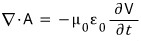
Let’s set div A like this — then a curious thing happens.​

​

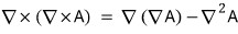
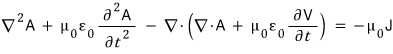
That strange-looking second equation from before

this

changes simply into this.

It seems like the Lorenz gauge is the div A that makes the middle term vanish to 0.

But the surprise doesn’t end there.

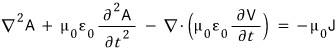
The first equation

this becomes

and this is,,,,,,,,,,

the vector potential A and the scalar potential V form exactly a symmetry.

That is

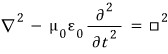
if we define one operator like this, we can describe the two equations above cleanly.

this operator is called the ’d’Alembertian operator’, apparently.

This Lorenz gauge is nice because it doesn’t violate causality, they say.

But there’s a drawback to the Lorenz gauge that I’ve picked out —

it’s aesthetically revolting T_T T_T T_T

Honestly, the very first time I saw it, I wanted to Skip it, but I read it sloooowly and found out it was no big deal, but….

Ughhh,.,…. a square-shaped operator suddenly showed up and I was so startled hehehehehelol it looks super difficulthehehehe

Anyway, when you work things out relativistically, writing V and A symmetrically like this is supposedly a good thing,

but right now I feel like I’m going to throw up….T_T T_T I think I’d better just go to sleep T_T… hehe

Originally written in Korean on my Naver blog (2015-08). Translated to English for gdpark.blog.