Binomial Model: One Period [Financial Engineering Programming #4]

So starting from Chapter 3, this is exactly where the Binomial Model shows up.

The reason it’s called ‘binomial’ is —

OK wait, let me back up first.

Realistically? People say predicting stock prices is straight-up impossible.

I mean… how would you even predict a stock price. Sounds like a totally absurd ask.

So people thought about it like this.

“OK fine, predicting the exact stock price is impossible. But still — couldn’t we at least figure out whether the price went up or down?!?!?!!!!?”

“Even if that was all we knew, we could invest with a clear head!!!”

So basically, the Binomial Model assumes that over any given period, a stock price is either in an ‘up state’ or a ‘down state’ —

it only takes those two states, builds on that idea, and tries to nail down the theoretical price of an option….

That’s why it’s called ‘binomial’, apparently.

More concretely:

“For a stock price, only two probabilities exist — the probability it goes up, and the probability it goes down. (Just like discrete probability in a coin flip!)”

So for now, we’ll only study the ‘one period’ case (one cycle… (?)).

Meaning we’ll only look at two points in time: right now, and at expiration. That’s what it boils down to.

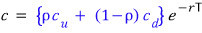
Now we’ll calculate the present value of a Call option over one period.

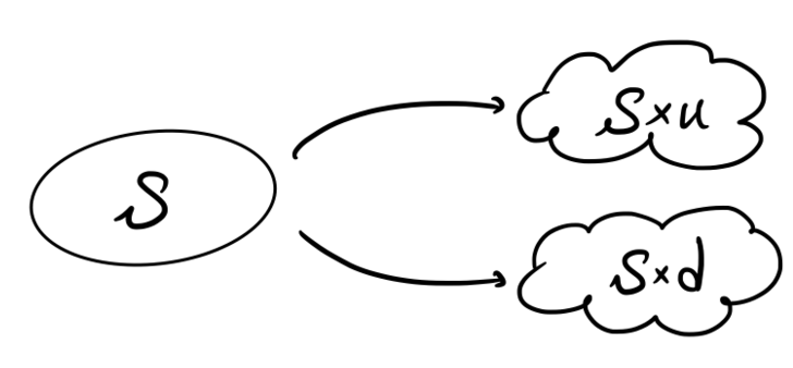
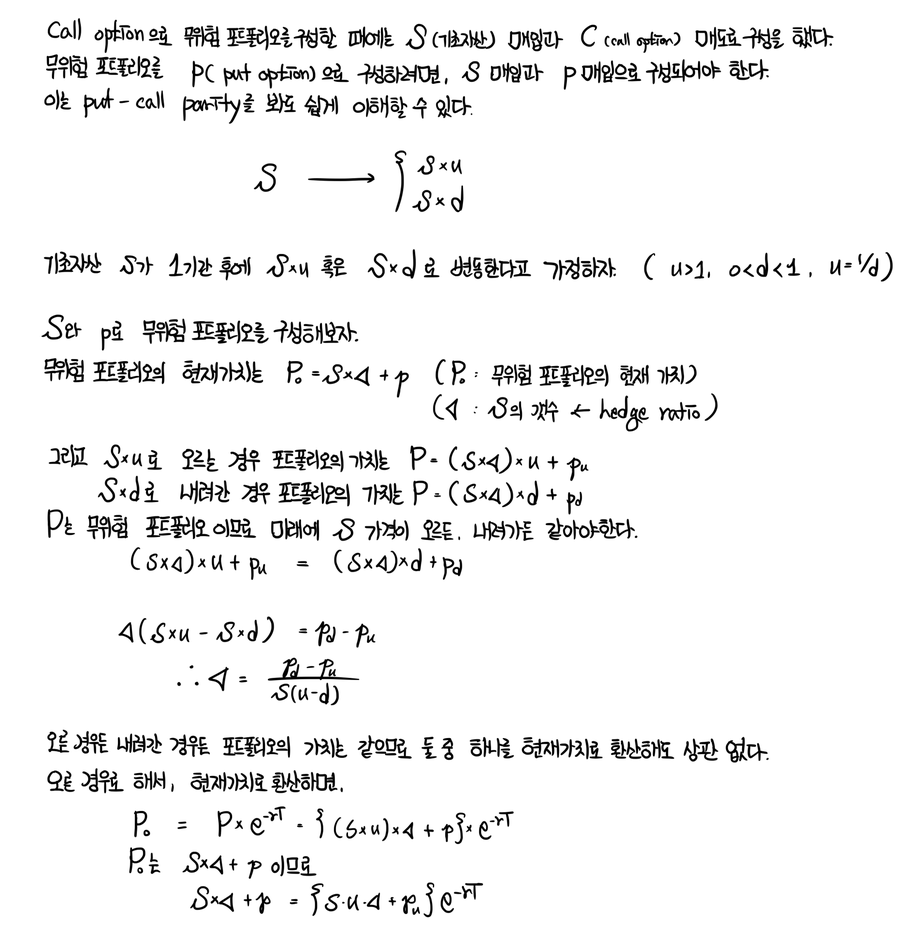
There’s an underlying asset whose current price is $S$,

and let’s say after one period it could become $S \times u$ ( $u > 1$ ), or it could become $S \times d$ ( $0 < d < 1 $ ).

And we’re going to build a risk-free portfolio —

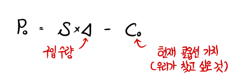
the portfolio’s gonna be: buy the underlying asset $S$, and sell a call option!

OK then, the current value of the portfolio

And the value of this portfolio one period in the future is

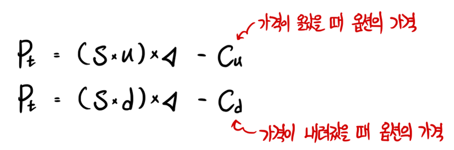
<$c_u$, $c_d$ — same thing as before: if $S \geq K$ then $c = S - K$, if $S < K$ then $c = 0$.>

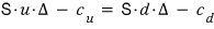
Since we built this portfolio as a risk-free portfolio, whether the price goes up or down,

the portfolio’s value has to stay the same after one period,

and so we can say the following equation holds.

Now if we mess around with this equation a bit

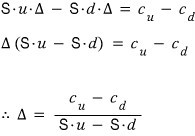
$\Delta$ is the number of shares we have to hold.

So this delta value is called the ‘hedge ratio’, apparently.

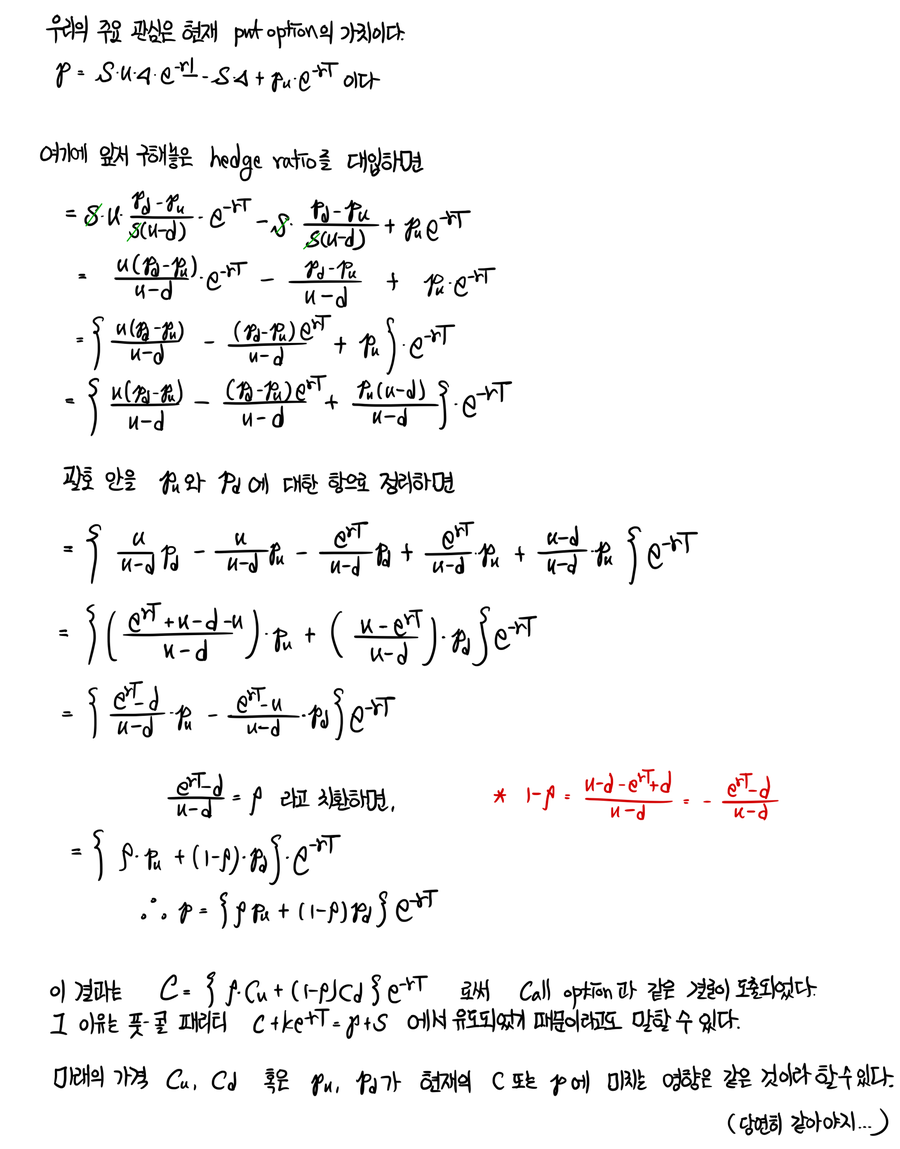
And — the value of this portfolio also has to equal the value from one period before!!!

That is, if we don’t want the word ‘risk-free’ to lose all meaning.

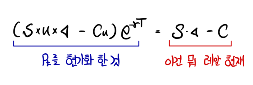
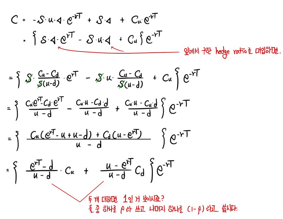
OK then,

That blue thing!! is the value before it’s been discounted to present value,

and we can call this thing ’the expected future value of $c$’.

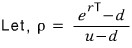
One thing to notice — it’s in the form of a ‘weighted sum’.

It’s gonna be an absolutely essential concept in the generalization work we’ll do later!!! Weighted sum! heh

Alright, I’ll write up the above as code real quick and then wrap this post up.

Sub Binomial_European_One_period()    'This is where I write the name of what I'm about to do.

Dim S as double, K as double, up as double, dn as double, rf as double, t as double, n as double

Dim rho as double, r as double, df as double, dt as double, c as double, cu as double, cd as double    'These are the names of the things I'm gonna use.

S=100: K=100: up=1.1: dn = up/1: rf = 0.05: t=1: n=1    'The relationship up×dn = 1 is one used in financial engineering — I'll bring it up again later.

dt = t / n

r = exp(rf * dt)

df = 1/exp(rf * dt)    'I think the reason they make a thing like a discount factor is just because it's handy when discounting to present value.

rho = (r-dn)/(u-d)

'These are my initial conditions~~

cu = Application.WorkSheetFunction.Max(S*up - K , 0)

cd = Application.WorkSheetFunction.Max(S*dn - K , 0)

c = ((rho)*cu(1-rho)cd)*df

End Sub

That red part — the Application.WorkSheetFunction. thing — is there because I wanted to use the Max() function that lives ‘in Excel’ from inside VBA, so I stuck Application.WorkSheetFunction. in front of Max().

If you drop the Application and just write WorkSheetFunction. it works the same, and

if you drop the WorkSheetFunction and just write Application. that also works, apparently —

but this might differ a bit depending on the version, so…. just take it as a rough guide T_T T_T T_T.

Anyway, the point is you can NOT just write cu = Max(s*up - K , 0) on its own!!!!

Because Max() isn’t a function that exists in VBA — it’s a function you have to drag in from somewhere else!!!!!!

lol lol

I also tried pricing a put option,

but suddenly I’m too lazy to type it all out —

and a few days ago someone showed me this very useful app….

So from here on out I plan to coast through the remaining posts of my life. lol lol lol lol lol

import numpy as np
import math
import matplotlib.pyplot as plt
import os

path = r'C:\Users\GD Park\Desktop\financial_engineering'
os.chdir(path)

def Binomial_European_One_period(S, K, up, rf):
    dn = 1/up
    t=1
    n=1
    dt = t/n
    r = np.exp(rf * dt)                  # For Exponential you can write math.exp(x), or pull in the one from numpy and use np.exp(x)
    df = 1/math.exp(rf * dt)             # 'df' stands for Discount Factor
    rho = (r-dn)/(up-dn)
    cu = max(S*up - K, 0)                # max is a built-in function!
    cd = max(S*dn - K, 0)
    c = (rho*cu + (1-rho)*cd) * df
    return c

Binomial_European_One_periodd = Binomial_European_One_period(S=100, K=100, up=1.1, rf=0.05)
print(Binomial_European_One_periodd)

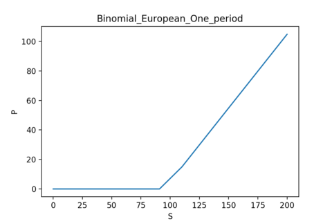
SS = np.linspace(0, 200, 1000)
YY = np.zeros(len(SS))
for i in range(len(SS)):
    YY[i] = Binomial_European_One_period(S=SS[i], K=100, up=1.1, rf=0.05)

plt.figure(figsize=(6, 4))
plt.plot(SS, YY)
plt.xlabel('S')
plt.ylabel('P')
plt.title('Binomial_European_One_period')
plt.savefig('Binomial_European_One_period.png', dpi=200)

Originally written in Korean on my Naver blog (2016-10). Translated to English for gdpark.blog.