Binomial Model: Generalized n-Period

So far we’ve done the one-period and the two-period binomial model.

Now it’s time to go full n-period.

In other words — generalization time.

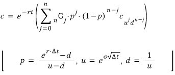
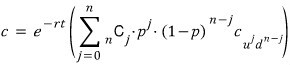
Let me just throw the generalized formula at you first.

Then I’ll go back and unpack it piece by piece, so

PLEASE do not panic when you see what I’m about to drop on you!!!!!!

※Warning: Heart attack risk ahead※

AAAA!!!!!!! My heart literally stopped… ;_; Ahhh…..

OK to make sense of this monster, let’s pull up the two-period formula one more time.

Phew… so why did that sigma (Σ) suddenly show up in the generalized version?!?!

Honestly, it’s just there to write the weighted sum in a compact way. That’s it.

Now let’s go through the new characters one by one before moving on.

First up: what is p?!?!?!?!?! Wasn’t there supposed to be a ρ (rho) sitting in that spot?!?!?!

• Originally, rho was written as

which we plugged in, and the meaning was something like: if ρ is the probability that the price goes up over period T, then (1-ρ) is the probability it goes down. Something like that.

But now we can’t talk about T anymore. Instead of “over T,” we have to say “over a unit of time.”

We take the whole T, slice it into tiny little pieces, and ask: does the price go up or down during this one little slice? —

That’s the lens we have to look through now.

Ah, OK, p is sorted. They just wrote p instead of the letter rho… heh.

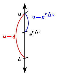
(But let me drop a quick word on why this thing can be interpreted as a “probability.” I think of it as something like a “geometric probability.”

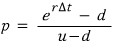
First, exp(rΔt) is the amount value automatically grows by (call it a multiplier).

u is the multiplier when it goes up, d is the multiplier when it goes down. So u-d is the total “size” of the move, and exp(rΔt)-d is the chunk of that u-d size that’s in the upward direction.

I’ll toss a little diagram down below. heh heh heh)

Second: what on earth is u?????

EXCUSE ME?!?!?!?!

Why is the up-rate u defined in that form, using σ and time —

apparently the answer to that question I cannot give you right now… ;; ;; ;_;

I’m sorry. My math is not strong enough yet. ;; ;;

(And honestly, volatility itself isn’t even a constant — it’s tangled up with other variables in really intricate ways… strictly speaking that’s the deal, but I can’t get into that right now either, so for now we’ll just treat it as a constant and crunch through problems.)

Third: u = 1/d

The reason for this lives inside the Cox-Ross-Rubinstein model… heh. heh.

Let’s punt the CRR model to next time.^^heh

Now, about that weighted sum —

it’s a simple object that anyone can read, but I still want to ramble about it for a sec before moving on.

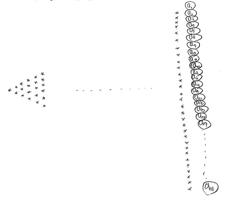
For example, say there are 31 possible option prices at exactly the maturity time T.

We need to take the weighted sum of those 31. That’s the whole job of the sigma.

So first off, with what probability does

— the value sitting at a_1 — actually show up?

Since it had to go up 30 times in a row, the probability is p^30.

(One period: 2 cases. Two period: 3 cases. So 31 cases means we’re in 30 periods right now.) And the number of ways this particular outcome can happen is 1.

But instead of just saying “the count is 1,” to really feel the weighted sum, it might be cleaner to write it as

cases.

What about a_2???? a_2 means: out of 30 price-move opportunities, it went down exactly once and up the other 29 times.

So the probability of landing on a_2 is (p^29)*(1-p).

And the number of ways this can happen — out of 30 opportunities, we just pick which 1 of them is the down move — so we get

cases.

One more at the end! Let’s just do a_17! Pure arbitrary pick!

a_17 is the option value after 16 down-moves and 14 up-moves out of 30 chances, so

the probability of landing on a_17 is (p^14)((1-p)^16), and the number of ways that can happen is

.

Phew.

OK so now the meaning of that weighted sum is also kinda… clicking, why it adds up the way it does!!! heh heh heh

PS

• The thing that becomes the weighted sum is

which is the price of the call option.

But I didn’t spell that out above, because the price of a call option —

it could be some number, sure, but it could also just be zero (because it’s nonlinear), so I just said “call price” and left it loose!!!

So among those, some entries could be zero. heh heh

import math
import numpy as np
import matplotlib.pyplot as plt
import scipy.stats as sc
import os
path = r'C:\Users\GD Park\Desktop\FinancialEngineering'
os.chdir(path)
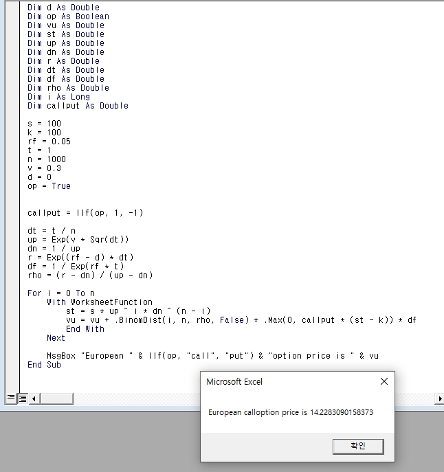
def Binomial_European_n_period(s=100, k=100, rf=0.05, t=1, n=1000, v=0.3, d=0, op=True, vu=0):
    dt = t / n
    up = math.exp(v * math.sqrt(dt))
    dn = 1 / up
    r = math.exp((rf - d) * dt)
    df = 1 / math.exp(rf * t)
    rho = (r - dn) / (up - dn)
if op == True:
        callput = 1
        callput_str = 'call'
else:
        callput = -1
        callput_str = 'put'
for i in range(n+1):
        st = s * (up ** i) * (dn ** (n - i))
        vu = vu + sc.binom(n, rho).pmf(i) * max(callput * (st - k), 0) * df
return vu, callput_str
vu, str = Binomial_European_n_period(s=100, k=100, rf=0.05, t=1, n=1000, v=0.3, d=0, op=True, vu=0)
print("European " + str + " option price is", vu)
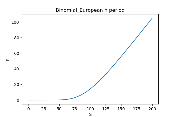
SS = np.linspace(0, 200, 1000)
YY = np.zeros(len(SS))
for i in range(len(SS)):
    YY[i], str = Binomial_European_n_period(s=SS[i])
plt.figure(figsize=(6, 4))
plt.plot(SS, YY)
plt.xlabel('S')
plt.ylabel('P')
plt.title('Binomial_European n period')
plt.savefig('Binomial_European n period.png', dpi=200)

Originally written in Korean on my Naver blog (2016-10). Translated to English for gdpark.blog.