American Options

Remember the American option I name-dropped a tiny bit earlier? Time to actually talk about it. Quick recap of what I said back then: the binomial model can price both European and American options. (The Black-Scholes formula only gives European prices in closed form, so for American options a tree like this one is the go-to tool.)

So… what’s actually the difference between the two?

Honestly? Just one difference. But it’s a chunky one. heh.

A European option can only be exercised at expiration. Only at expiration. End of story. An American option? Exercise whenever you want. Any time before expiration is fair game. Early exercise — totally allowed.

(I don’t really know the history here, but doesn’t America have a bit of a gangster vibe? lol. The whole “if things aren’t going my way I’m pulling the trigger right now” energy. lol lol)

OK so before, at the very~~~ end of the tree, we had which was $S \cdot u^{j}d^{n-j} - K$ or zero.

One of the two values got locked in, we present-valued it, and swoosh — added everything up. Right?! But now that whole picture changes.

For a European option, the path doesn’t matter. Whatever the value was at intermediate nodes — doesn’t matter. If it ended up at zero by expiration, the whole path is just zero. Done.

But for an American option:

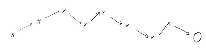
among these nodes — a path can be worth something partway along and still end at zero. Does that mean you should have exercised back there? Nobody can see the next branch in advance, so at every node the holder compares exercising right now with the discounted value of holding on, and takes the larger. Standing at a node like that, you might catch yourself thinking:

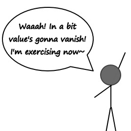
So we have to check the call value at every single node.

The person sitting at each node is thinking:

“Hmm… should I exercise now? Or hold?”

“If I exercise right now vs. what’s the expected value at the next step from here?” That’s the call they’re making.

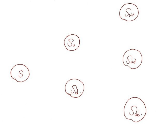
OK so each point in time has its own situation. The folks sitting at expiration? They’ve got nothing to compare against — there’s no next step. So they just go with $\max(S_{ud} - K, 0)$. No choice.

But the folks in the middle…

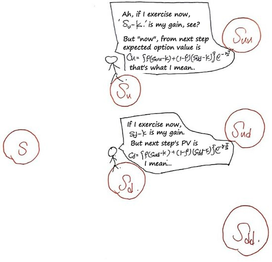
Yeah, there’s gonna be a lot of chatter at these nodes. So much chatter, for real. lol

If you’re not at expiration yet, you compare against the expected call value in the next state — and pick whichever is higher.

You’d compare against the present-valued option value at that point… heh.

(Or equivalently: take the immediate exercise value $S_u - K$, future-value it, and compare against the value at expiration. The formula handles both ways of thinking. Same thing.)

Honestly, this whole thing is way easier to feel through code.

So if we write code a certain way, can it represent the current $c$ for the situation above?

Quick high-level: you do the option pricing from the very back and walk toward the start of the tree. Nobody can see which branch comes next, so at each node you compare exercising right now with the discounted expected value of holding on, and keep the larger one. Code for that situation looks like this. heh.

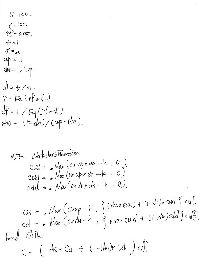
Sub ~ End Sub. But you can also build a tree where you can see the whole interval at once.

Don’t try to write the full thing right out of the gate. First let’s look at how to build a tree with code, get how the tree gets put together, and then we’ll do the option price tree!! heh.

So, first up — coding a simple tree looks like this. I’ll skip the variable declarations.

n=5: k=0:
For i=n To 0 step -1
    For j=i To 0 step -1
        k = k+1
        Cells(2 * j + ( n - i ) + 1, i + 1) = k
    Next
Next

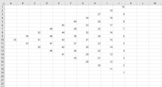
If you just run this, a tree shows up on the sheet. Done. But honestly? I had a hard time with this at first. So I went full brute-force interpretation mode…… (T_T)

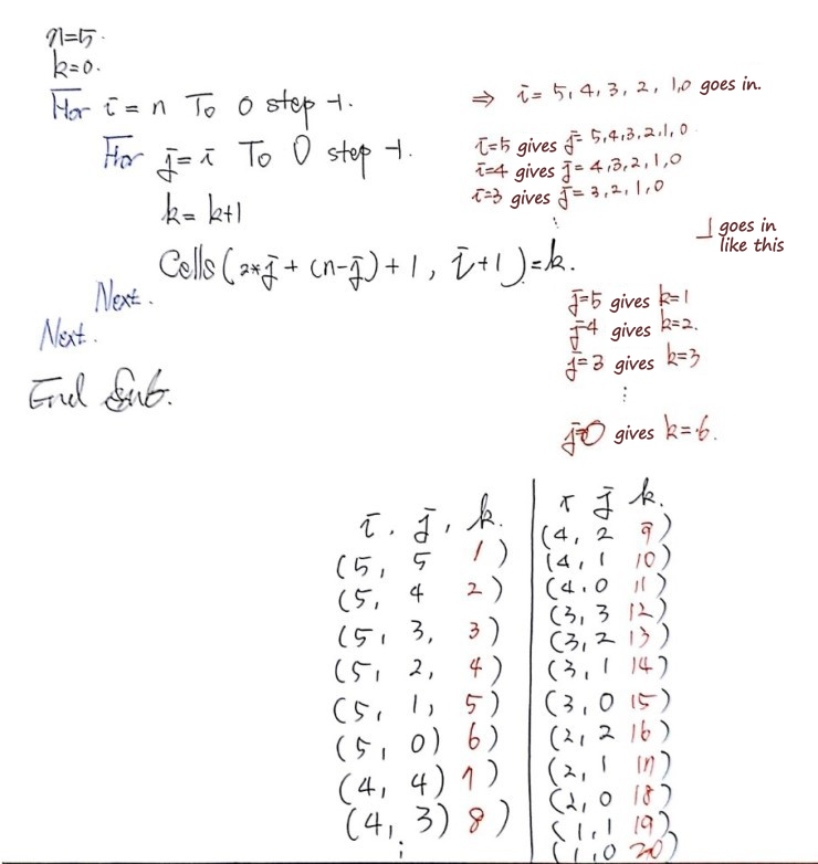
First I looked at how j changes when one i goes in, and how k changes each time j changes. Then, to see how this maps into the Cell coordinates, I matched up the i, j to each Cell. In that order, the Cell gets k = 1, 2, 3, 4, 5, 6, ... written into it.

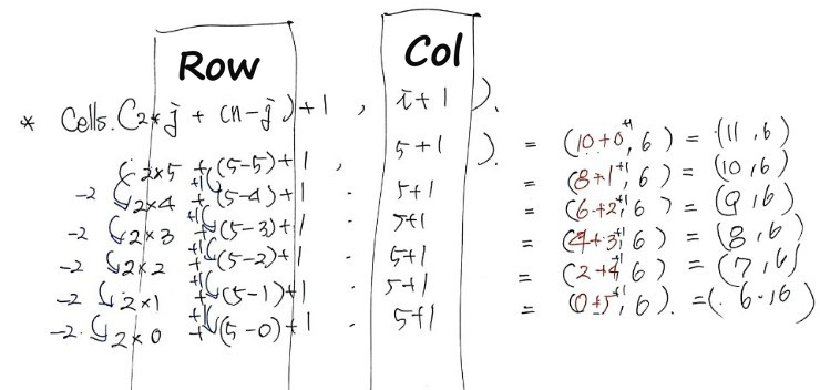
After working through this much, the pattern clicked, so I stopped. Turned into one shape only at $i=5$. heh. OK. So we roughly get how the tree is drawn.

Now let’s code it so Excel draws the binomial tree we drew earlier. Aaaaahh — well, not us doing the coding from scratch, but us looking at the already-coded version and trying to understand it!

S = 100: k = 100: rf = 0.05: t=1: n=5: up=1.1: dn=1/up:
dt = t/n: r = exp(rf*dt): df = 1/r
rho=(r-dn)/(up-dn)
z=0
With WorkSheetFunction
For i=5 To 0 step -1
    For j=i To 0 step -1
        if i=n then
            z = .Max((up)^(i-j)*(dn)^(j)*S - K, 0)   'i=5 means we're at the very end
        elseif 0<i and i<n then
            z = .Max((up)^(i-j)*(dn)^(j)*S - K, (rho*cells(2*j+(n-i), i+2) + _
                (1-rho)*cells(2*j+(n-i)+2, i+2))*df)
        else
            z = (rho*cells(2*j+(n-i), i+2) + (1-rho)*cells(2*j+(n-i)+2, i+2))*df
        End if
        cells(2*j+1+(n-i), i+1) = z
    Next
Next
End With

Before reading the if / elseif / else, let’s first look at Cells( ~ ) — the part that tells us where each i, j lands. Here’s how I worked it out:

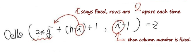
Then,

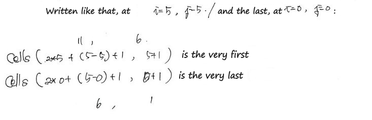
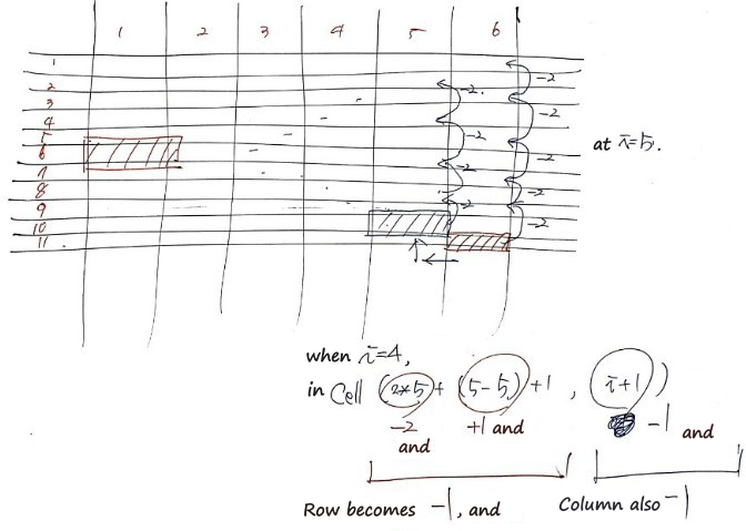
Oh — now I see how what’s getting written can actually be written as a tree.

Now the conditionals. I get why i = n is its own case. At expiration it’s $\max(\text{something}, 0)$. Whereas for $0 < i < n$ (here $i = 1, \dots, 4$), it’s $\max(\text{something}, \text{something else})$.

But why does the very first initial point — i = 0 — also need its own else branch?

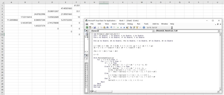
Because in this example exercising right at the start would pay less than holding on, so the code skips Max() there and just discounts the expected value. (In general an American option can be exercised right away too, so a full tree compares $S - K$ with the discounted value at every node, the first one included. For a call on a stock that pays no dividends that comparison never picks early exercise, which is why the American call here comes out at the same 11.3266 as the European one.)

import pandas as pd
import os
path = r'C:\path\to\your\folder'   # wherever you keep the files
os.chdir(path)
name = 'make a simple tree'
# make a tree with n slots
n=10; k=0
n_col = [x for x in range(0, 200)]
n_row = [x for x in range(0, 200)]
df = pd.DataFrame(columns=n_col, index=n_row)
for y in range(n, 0, -1):
    for x in range(y, 0, -1):
        k+=1
        df.loc[2*x-1+(n-y), y] = k
df.dropna(how='all', inplace=True, axis=0)
df.dropna(how='all', inplace=True, axis=1)
writer = pd.ExcelWriter('make a simple tree.xlsx' , engine='xlsxwriter')
df.to_excel(writer, sheet_name='make a simple tree')
writer.close()

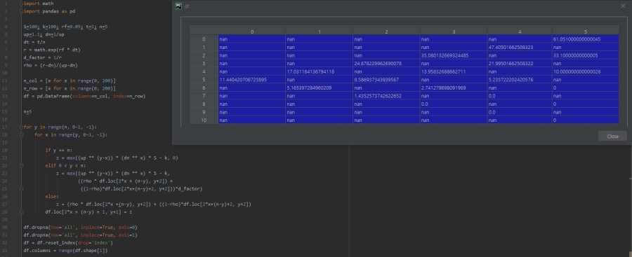
import math
import pandas as pd
S=100; k=100; rf=0.05; t=1; n=5
up=1.1; dn=1/up
dt = t/n
r = math.exp(rf * dt)
d_factor = 1/r
rho = (r-dn)/(up-dn)
n_col = [x for x in range(0, 200)]
n_row = [x for x in range(0, 200)]
df = pd.DataFrame(columns=n_col, index=n_row)
n=5
for y in range(n, 0-1, -1):
    for x in range(y, 0-1, -1):
        if y == n:
            z = max((up ** (y-x)) * (dn ** x) * S - k, 0)
        elif 0 < y < n:
            z = max((up ** (y-x)) * (dn ** x) * S - k,
                    ((rho * df.loc[2*x + (n-y), y+2]) +
                     ((1-rho)*df.loc[2*x+(n-y)+2, y+2]))*d_factor)
        else:
            z = ((rho * df.loc[2*x +(n-y), y+2]) + ((1-rho)*df.loc[2*x+(n-y)+2, y+2])) * d_factor
        df.loc[2*x + (n-y) + 1, y+1] = z
df.dropna(how='all', inplace=True, axis=0)
df.dropna(how='all', inplace=True, axis=1)
df = df.reset_index(drop='index')
df.columns = range(df.shape[1])

Heads-up. The figures here are the original notes, slips and all. A few things to watch for:

• One handwritten sketch writes (n-j) in the row index where the code and the later pictures use (n-i).
• The Python output in the screenshot (11.4404… at the first node) comes from a version that forgot to discount the first node; with the discount, as in the code above, it gives 11.3266, the same as the Excel tree.
• The stick figure who says the value is about to vanish is a prompt for intuition, not a forecast: nobody knows the next move, and the decision at each node compares exercising now with the discounted expected value of holding.