Wiener Process [Financial Engineering Programming #8]

Alright, Chapter 4 — the Black-Scholes model.

Before I even start, let me tell you what I already know in my bones: I am not going to understand the Black-Scholes model right here in this blog post. lol

Also, I absolutely cannot derive Black-Scholes. Like, not even close. lol lol lol

So what I’m gonna do is just take the already-built Black-Scholes formula and code it up. That’s it. That’s the post. T_T

If anyone clicked in here hoping for some big deep enlightenment moment… I’m telling you upfront — heh, sorry.

OK then, let’s go.

I’m gonna follow the book as faithfully as I can, and the actually-grasping-Black-Scholes-properly part? We’ll save that for grad school. Grad school. lol

So. Stock prices clearly move in some random way, right?

If there were any kind of sequential rule to them, somebody would’ve already —

no, like a million people would already be billionaires.

But also — while they move randomly, it’s not like the price suddenly jumps from +1893081094810984109

to, out of nowhere, 10.

That kind of insane garbage doesn’t happen. So it’s not fully random — it’s random within some kind of model for stock prices.

And to evaluate options on stocks, we need that model. We need a “model for stock prices.” Apparently.

So people went hunting for one, and the model that ended up best capturing the statistical behavior of stock prices is the Geometric Brownian Motion model.

Wait!?!?!? Brownian motion — is that the one I’m thinking of???

Take a look sometime: ( http://gdpresent.blog.me/220750324668 )

Brownian motion — with the Langevin equation [ stuff I studied… ]
Around middle school??? You probably ran into Brownian motion. At school you dropped a drop of ink — splosh — into water, right???? How does liquid…
gdpresent.blog.me

That post is the simple physics-side explanation of Brownian motion, but the same idea later flowed into Samuelson’s work and became Geometric Brownian Motion, which ended up playing a starring role in stock pricing. Apparently.

(For the history, this is a good read: http://blog.naver.com/ketema/39957447)

Ah… but going off and reading all those is a bit inefficient, so let me just briefly cover Brownian motion right here.

Brownian motion — in 1905, the miracle year, Einstein dropped 4 papers.

(All 4 were so insane that 1905 just got named “the miracle year.” lol)

One of those four is the special relativity paper — everyone knows that one now, thanks to Interstellar. Another one was on Brownian motion. Another was on mass-energy equivalence ($E=mc^2$). And the last one was on the photoelectric effect — the one that basically birthed quantum mechanics. Yeah. Miracle year is right.

Anyway, Brownian motion gets born like that, and after WWII ends, it migrates over to an economist. And that’s where it morphs into Geometric Brownian Motion.

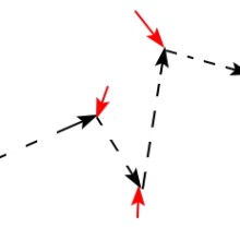
Brownian motion just refers to all kinds of random motion happening around us. Easy version — middle school version — drop ink into water. The way the ink spreads out (random, right?). That’s the vibe.

When people applied this model to the stock market, turns out it explained things well enough.

So before we apply Brownian motion to the stock market, we lay down some assumptions first:

Stock prices are uncertain. You can know today’s price; nobody knows tomorrow’s.
Changes in stock prices are continuous.
Stock prices follow a log-normal distribution.
Stock returns follow a normal distribution.
The expected return of a stock and the uncertainty of its return are both proportional to the holding period.

(A log-normal distribution is what you get when you exponentiate a normal distribution — and doing so gives you a distribution where the mode is skewed to the left. Apparently.)

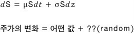
Lay down those assumptions, and the stochastic process model for stock prices under GBM is:

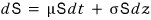
$S$: stock price
$\mu$: expected return of the stock price
$\sigma$: volatility of the stock price lol

$\mu$ and $\sigma$ — these are technically variables, but we’re going to assume they’re constants.

** $z$: random variable (The random variable $z$ follows the Wiener process.)

Wiener process: a stochastic process where the mean of the changes in the variable is 0 and the variance is 1.

I’m weak at math, so I think I need to dig into “random variable” a little more before moving on. T_T What even is a random variable, seriously… T_T ugh…….

Random variable:

A variable that assigns a numerical value to events that occur with some probability. Generally denoted $X$.

When you do an experiment or observe some phenomenon involving randomness, and a single real value $X$ shows up as the result — $X$ is a “variable” in the sense that it could’ve taken many possible values, but which value it takes and with what likelihood is described by the probability defined for it.

That’s a random variable.

Random variables come in two flavors: discrete random variables (finite number of possible values) and continuous random variables (infinite number of possible values).

OK, I just kind of copied that out for the random variable $z$.

So basically — when variable $z$ wiggles around wildly~~~~~~~~~, that wiggling is determined probabilistically. And the Wiener process means the trend of that wiggling follows a distribution where the mean is 0 and the variance is 1.

Cool. Then,

This formula? Yeah, no way I’m proving this here lol lol lol lol

I keep telling you I’m not a math major. lol lol lol lol T_T sad

I want to be good at math too T_T

Let’s loosely — no no — very loosely understand this formula and move on.

$dS$ is the change in the stock price. Change. (the $d$ as in $\Delta S$.)
$\mu S\,dt$ is the expected value of the instantaneous change in stock price during a tiny time $dt$.
$\sigma S\,dz$ — and this is where the trouble is… heh

Since the random variable $z$ follows the Wiener process, “the change in $z$” — that is, $dz$ — is determined by that probability distribution with mean 0 and variance 1.

So we can write:

In other words — the change in stock price is random, but

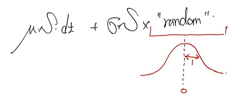
it’s not, like, super-random.

Ah, but in the actual stock market, observing $dS$ in practice is hard. What I mean is — measuring $dS$ over the unit time $dt$ (i.e., continuously, for all values) is a pain. So we look at $\Delta S$ over $\Delta t$ intervals instead of exactly $dt$.

From that angle, mathematically(?), $\Delta z$ has the property:

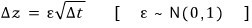
like that, apparently. $\varepsilon$ is a number — a random number drawn from $N(0,1)$.

(This relationship is what Wiener showed, and we just use it. heh)

OK so I’m slowly going to start coding, but before that, let me organize a couple of things that are gonna get confusing as I keep going.

-dist: cumulative distribution value
-Inv: cumulative probability

Later we’ll use a function called NormSInv, so let me get the why of “inverse” straight before moving on.

I’ll lay out these 4: NormDist, NormSDist, NormInv, NormSInv.

NormDist(x, mean, std): probability that the random variable comes out as $x$ or less, given a mean and standard deviation.

e.g. NormDist(10, 36, 21) = 0.1078
→ In a normal distribution with mean 36 and std 21, the probability of getting 10 or less is 10.78%.

NormSDist(x): probability of getting $x$ or less in the standard normal distribution ($\mu=0$, $\sigma=1$).

e.g. NormSDist(0) = 0.5
→ In the standard normal, the probability of getting 0 or less is 50%. Yep.

NormInv(prob, mean, std): the inverse direction — given a cumulative probability, what’s the random variable value, in a normal distribution with that mean and std?

e.g. NormInv(0.14, 35, 14) = 19.87553
→ In a normal with mean 35 and std 14, the $x$ at which the cumulative probability hits 14% is 19.87553.

NormSInv(prob): yeah yeah yeah yeah easy mode… too lazy to type more.

e.g. NormSInv(0.94) = 1.55474
→ In the standard normal, the $x$ at which you’ve hit 94% is 1.55474.

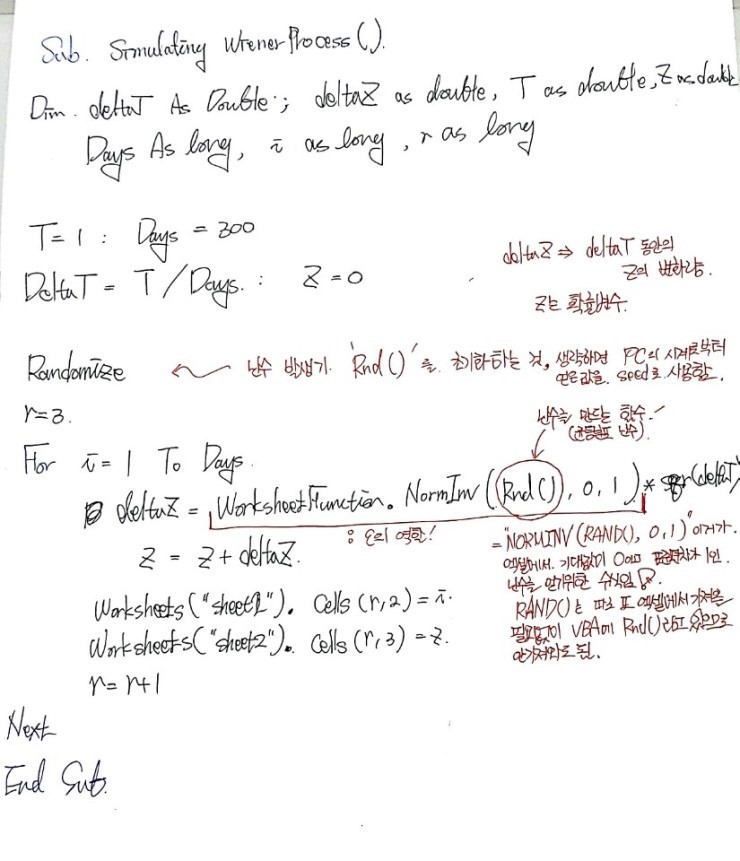
OK. Now let’s just code up the Wiener process the way the book does it, and call it.

We need to draw a random number $\varepsilon$. Now, if we just draw with Rnd(), we get a random number between 0 and 1 — but the catch is, when $a$ and $b$ both come up, they come up with equal probability.

A number drawn like that is not a number drawn following the Wiener process.

What kind of number do we actually need?

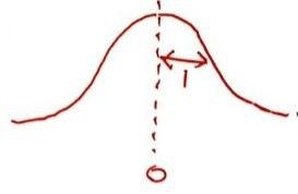
We need a number drawn from this kind of distribution — meaning even if $a$ and $b$ both can show up, they should each show up with different probabilities.

So now you can see why Δz = Rnd() * sqr(deltaT) won’t cut it in the code, right?

That’s exactly why we have to draw the random variable $z$ as NormInv(Rnd, 0, 1) or NormSInv(Rnd()). heh.

import numpy as np
import math
import pandas as pd
import matplotlib.pyplot as plt
import os

path = r'C:\Users\GD Park\Desktop\금융공학'
os.chdir(path)

T = 1; Days = 300; deltaT = T/Days; z=0

n_col = [x for x in range(0, 500)]
n_row = [x for x in range(0, 500)]

df = pd.DataFrame(columns=n_col, index=n_row)

np.random.seed(2000)

for x in range(1, 301):
    deltaZ = np.random.normal(loc=0, scale=1) * math.sqrt(deltaT)
    z = z + deltaZ
    df.loc[x, 1] = z

df.dropna(how='all', inplace=True, axis=1)
df.dropna(how='all', inplace=True, axis=0)
df = df.reset_index()
df.columns = range(df.shape[1])

plt.figure(figsize=(6, 4))
plt.plot(df.T.iloc[0].values, df.T.iloc[1].values)
plt.savefig('Wiener Process.png', dpi=200)

Originally written in Korean on my Naver blog (2016-10). Translated to English for gdpark.blog.