Monte Carlo Method

The Monte Carlo method is…

hmm… “the more you do it, the closer you get to the average.”

Feels kinda like the law of large numbers, right?

Back in the day when I was shepherding high school kids around campus, walking them from department to department for major intros — when I dragged them into the statistics department —

that’s where they explained this “Monte Carlo Method.”

And dang, I caught myself actually paying attention lol lol lol lol

Up till then I’d only ever heard the name and had no real clue what it was, but those stats students broke it down clean lol lol lol

So first — Monte Carlo is one of the four districts (區) that make up Monaco. It sits across the harbor from the capital, Monaco City. It blew up as a Mediterranean tourist/resort spot after Prince Charles III of Monaco gave the green light to open a casino.

In 1866, it got renamed from Sverip.

As Monaco’s main commercial district, it’s packed with hotels, theaters, apartments, and it hosts car races, sports festivals, that kind of thing.

[Naver Encyclopedia of Knowledge] Monte Carlo (Dictionary of World Place Name Origins, 2006. 2. 1., Sungji Munhwasa)

Apparently it’s a city famous for gambling.

And now, in academia —

this “Monte Monte” thing — which apparently got its start during the atomic bomb project — in the simplest possible terms:

(for the actual details, hit Wikipedia or some other blog.)

It’s one of those computer simulation methods. You basically tell a computer to scatter a crap-ton of dots at random.

Just — fire away, randomly.

You can absolutely make a computer plot dots randomly.

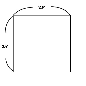
Run it dead simple, and when the computer drops 5,000 dots,

it counts how many landed inside the square. Apparently around 1,917.

OK now, which dots are we counting —

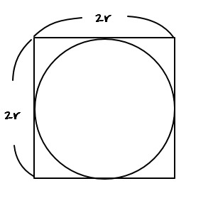
we count the dots that fell inside a circle of radius r, like this.

When you count, apparently about 1,503 get caught.

And then when you take the ratio:

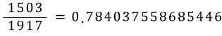
You get this. And what we just calculated is…. (https://playentry.org/thdtkdtn/55532f8d3fad2adb3767e7d7#!/)

Apparently that’s what we calculated…..

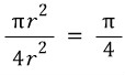
Whoa. So what happens if we multiply by 4…?

Yep…. apparently you can compute π this way.

We’re not at 3.14 yet, but they say if you crank the number of trials up more and more and more and more and more and more, you can pin down the ratio to a truly astonishing degree.

(Yeah. I tried it lol lol lol lol)

https://gdpresent.blog.me/221660360230

Calculating pi using the Monte Carlo method (Calculate pi by using Monte Carlo Method)

https://www.youtube.com/watch?v=BZdbuBBW-1A It’s slow when you actually run it~ the video is though lol lol lol so…

gdpresent.blog.me

……..Are you starting to get a feel for what the Monte Carlo method is going for???????? lol lol lol lol lol

So I want to use that kind of method here — but not with the formula from before. With a different one.

Quick recap before we move on, though.

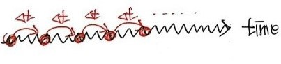
Brownian motion from physics, when it crossed over into the financial world,

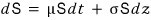
morphed into this. And

in real life, measuring something like dt or dS — that kind of crazy-tiny infinitesimal change — is basically impossible,

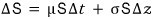
so I figured: change dt, into something a bit chunkier, Δt, and dS into ΔS.

So I just went ahead and swapped them. Boldly.

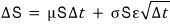
After that swap, a gentleman named Wiener —

a gentleman who is not a loser — proved through statistical properties that

we get this property. (And ε ~ N(0, 1).)

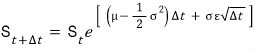
So the finished formula came out as

and we even coded it up.

But — turns out that one was wrong.

Because the formula that was truly derived in the first place is

this one, and

measuring it this way is the “real deal,”

but jamming this true formula into

this one

meant the measurement was actually being done

like this sloppy mess. Which is exactly where the error sneaks in…

So — using the famous Itô’s Lemma —

apparently you can get a more accurate formula, and that one looks like

Let’s just accept this as “a slightly more accurate version of GBM than before” and keep moving!

Now to actually see how the two values differ from each other,

we can code it up and check with our own eyes.

Shall we?

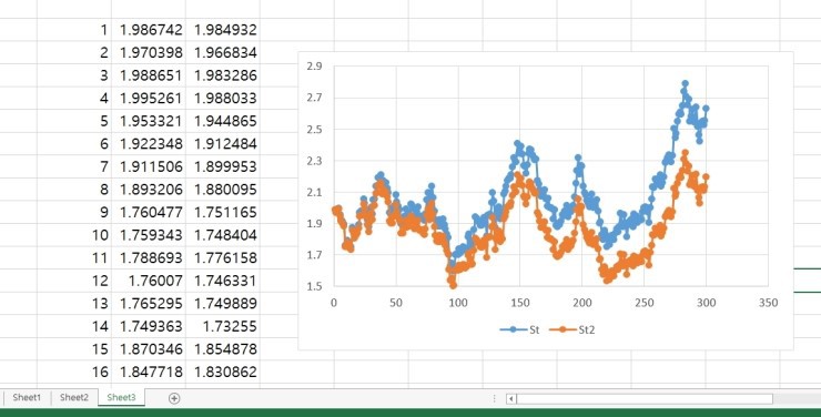
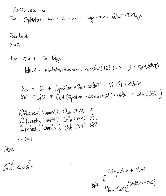
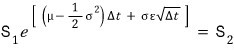
Same starting value,

St is the old Wiener process,

and St2 is today’s allegedly-more-accurate version. Blue and orange.

And now, if we use the Monte Carlo method with the new (supposedly-more-accurate) formula to predict a stock price, here’s what we get:

Sub monte_carlo_thing ()

    Dim ~~~~~~~~~~ugh, lazy~~~~~~~ as Double

    S = 100: v = 0.3: r = 0.15: T = 1: iter = 5000
    vvt = v*v*T

    For i = 1 To iter

        this_Gaussian = worksheetfunction.NormSInv(Rnd())
        this_spot = S * exp(r*T - 0.5*vvt + sqr(vvt)*this_Gaussian)
        running_sum = running_sum + this_spot

    Next

    mean = running_sum / iter

    Debug.Print mean

End Sub

Setting v — volatility — to 0.3 as the standard deviation of returns, fine, no surprises there.

But I was kinda curious why the expected return μ got written as r specifically,

and apparently if you keep going further along, you find out expected return and the risk-free rate are basically the same thing.

In the code above, this_Gaussian

is just the same NormInv(Rnd(), 0, 1) thing from before,

and this_spot is the “change” after one period from $S_0$.

After we run For → Next, i bumps to 2,

and once we have $S_1$, then for that $S_1$ again

it becomes this again, becomes this_spot again, gets added to running_sum,

then through Next again — $S_3$ gets made off of $S_2$, added to running_sum,

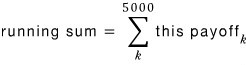
and as 5,000 this_spots pile up into running_sum like that,

at the very end, all 5,000 get divided by 5,000 to get the average!!!

And that’s what we call mean!!!

Eek!

What does it mean….

Here’s how I’m thinking about it.

Like before — instead of trusting some single $S_t$ that fell out of running the simulation once,

run it 5,000 times —

no, 10,348,319,840,913,890,438,109,809 times — and trust the average of all those. That feels more trustworthy….. yeah, something like that is what I’m getting at.

Using the Monte Carlo method (which carries this philosophy),

this time let’s also try estimating the price of a Call option.

But — eh, nothing too wild, since C = S − K… heh.

I’ll just throw the code at you again.

Function monte_carlo_Euro_call (S, k, r, v, T, iter) As Double

    Dim ~~~~~~~~~~~~~~~~~~~~~~~~~~~~~~~~~~ As Double
    Dim ~~~~~~~ As Long

    S = 100: v = 0.3: nu = 0.15: T = 1: iter = 5000

    For i = 1 To iter

        this_Gaussian = worksheetfunction.NormSInv(Rnd())
        this_spot = S*exp(r*T - 0.5*vvt + sqr(vvt)*this_gaussian)
        this_payoff = this_spot - k
        this_payoff = iif( this_payoff > 0, this_payoff, 0 )
        running_sum = running_sum + this_payoff

    Next

    mean = running_sum / iter
    monte_carlo_Euro_call = mean*exp(-r*T)

End Function

OK first thing — we need to distinguish between Sub procedures and Function procedures,

because the one above isn’t a Sub like everything we’ve done so far. It’s a Function.

Sub procedure: think of it as a function, but no return value.

Function procedure: this one has a return value.

I think it’s enough to just file it away as “the one with a return value” and move on.

So inside the For loop up through this_spot, it’s exactly the same as before — it’s plotting the stock changes one by one,

and on top of that we added this_payoff and slapped a condition on it.

So when i = k,

if we say that, then running_sum is

this. But each individual

has to pass the “is it positive?” check to have a value,

and when something negative pops out, we just shove it to 0, so among all those

there’ll definitely be some zeros mixed in. That’s the deal.

Anyway,

with those mixed in too,

we sum up all the

and take the average lol lol lol lol lol.

That average then gets discounted back to present value at the end,

and the return value of the declared Function gets defined as exactly that.

And the book takes this Function we just built and uses it inside another Sub procedure,~~~~

Looks like we’ll have a chance to actually use it when we get to the 5 Greeks.

That’s it for today!

Originally written in Korean on my Naver blog (2016-10). Translated to English for gdpark.blog.