Black-Scholes Formula

The title is flashy, so let me cut to the chase real quick.

I cannot derive Black-Scholes!!! lol lol lol

If you came here to learn how the derivation works — please, leave, immediately, lol lol lol

I’m just gonna focus on coding the Black-Scholes model. That’s what this post is about.

So first, let me throw down the “Black-Scholes PDE (partial differential equation)” — yeah, the one that won the Nobel Prize in Economics.

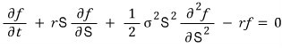
That right there is the Black-Scholes partial differential equation, the Nobel-Prize-in-Economics one.

But — the formula I’m actually going to use here? Not that one.

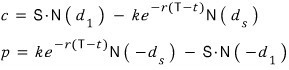
The thing you can get by solving that PDE — using some seriously advanced math — is the Black-Scholes option pricing formula…

So really, the Black-Scholes option pricing formula is more like a Fields Medal kind of thing — the Fields Medal being the “Nobel of math,” not the actual Nobel —

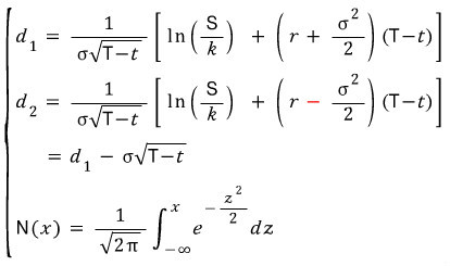
Alright, so let’s run through the assumptions baked into the Black-Scholes model,

and then I’ll go ahead and crunch a call and a put using the formula above.

i) There is no arbitrage opportunity

(no way to make a riskless profit)

······· “no arbitrage opportunity”

ii) You can borrow and lend any amount

(even fractional, of cash, at the riskless rate)

······· any amount of cash, you can borrow or lend it, no problem

iii) You can buy and sell any amount

(even fractional, of cash, at the riskless rate)

······· buying or selling any amount of stock is also fine

iv) The above transactions don’t incur any fees or costs

······· no transaction costs, no fees (perfect market)

v) The rate of return on the riskless asset is constant

······· the riskless rate is a constant

vi) The stock price follows a geometric Brownian motion,

and we’ll assume its drift and volatility are constant

······· the stock price is Brownian, with drift and volatility taken as constants

(how should I think of “drift” here — like the current pulling the stock along, or the stock’s tendency to move? I’m not totally sure what to call it.)

Oh, and one more important thing in BS: you only need the volatility of the stock, not its expected return. That’s apparently the big insight… heh?

OK, now let’s just go ahead and

use the dang thing.

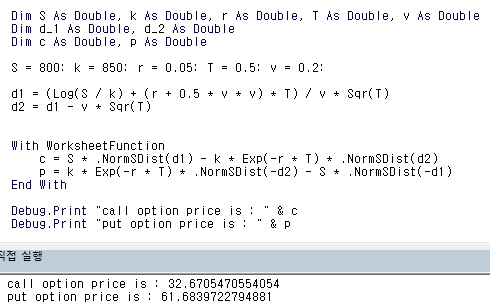
S = 800: k = 850: r = 0.05: T = 0.5: v = 0.2:

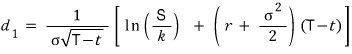
d_1 = (log( s / k ) + (r + 0.5*v*v)*T / v*sqr(T))
d_2 = d_1 - v*sqr(T)

with worksheetfunction

c = S*.NormSDist(d_1) - k*exp(-r*T)*.NormSDist(d_2)

p = k*exp(-r*T)*.NormSDist(-d_2) - S*.NormSDist(-d_1)

End with

debug.print "call option price is : " & c

debug.print "put option price is : " & p

End sub

Deriving the formula is hard. Coding it once you have the formula? Not hard at all.

If you think real loosely about what $N(d_1)$ even is —

what $N(x)$ means is:

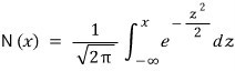
That’s the definition,

so it’s the probability that a standard normal $N(0,1)$ spits out a value less than or equal to $x$.

Then $N(d_1)$ is, like… weirdly:

The cumulative probability of getting a value less than or equal to that number is $N(d_1)$? OK?

But like… what does that even do for us T_T I don’t know what the numbers $d_1$ and $d_2$ actually mean T_T

For now I just gotta remember it like this,,, T_T T_T T_T

import numpy as np
import scipy as sp
import scipy.stats
import math
import matplotlib.pyplot as plt
import os

path = r'C:\Users\GD Park\Desktop\financial_engineering'
os.chdir(path)

def BS_Formula(S=800, k=850, r=0.05, T=0.5, v=0.2):
    d1 = math.log(S/k) + (r + (v*v)*0.5)*T
    d1 = d1 / v*math.sqrt(T)
    d2 = d1 - v*math.sqrt(T)
    norm = sp.stats.norm(loc=0, scale=1)
    c = S*norm.cdf(d1) - k*math.exp(-r*T)*norm.cdf(d2)
    p = k*math.exp(-r*T)*norm.cdf(-d2) - S*norm.cdf(-d1)
    return c, p

SS = np.linspace(700, 900, 1000)
C = np.zeros(len(SS))
P = np.zeros(len(SS))
for i in range(len(SS)):
    C[i], P[i] = BS_Formula(S=SS[i])

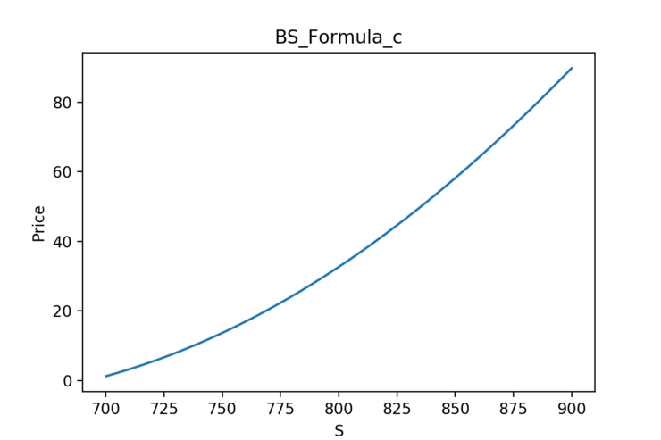
plt.figure(figsize=(6, 4))
plt.plot(SS, C)
plt.xlabel('S')
plt.ylabel('Price')
plt.title('BS_Formula_c')
plt.savefig('BS_Formula_c', dpi=200)

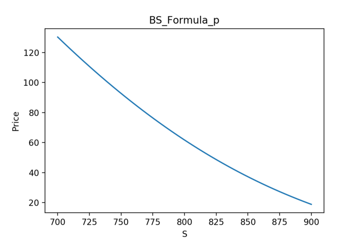
plt.figure(figsize=(6, 4))
plt.plot(SS, P)
plt.xlabel('S')
plt.ylabel('Price')
plt.title('BS_Formula_p')
plt.savefig('BS_Formula_p', dpi=200)

Originally written in Korean on my Naver blog (2016-10). Translated to English for gdpark.blog.