Bisection Method & Weighted Bisection Method [Financial Engineering Programming #14]

Alright, from here on out we’re playing the “find-the-solution” game.

First up: of all the ways to find the root of an equation on a computer, the easiest one is the Bisection Method —

and I mean extremely easy!!!

OK, the basic idea of the bisection method is

right here.

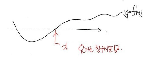
This is what we want to find — like, right now:

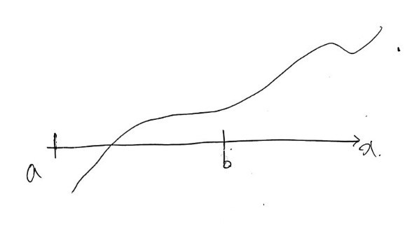
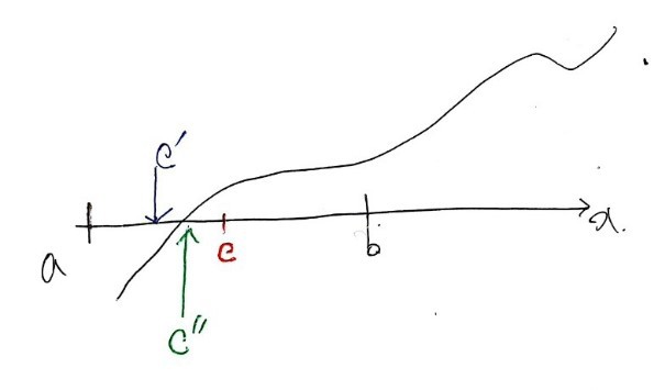
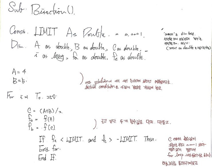
First, let’s say we pick our initial values $a$ and $b$ like this.

(Wait, what??? Just keep reading, you’ll see what I mean.)

Why those particular $a$ and $b$ as starting values?

Because we pick them so that $f(a)$ and $f(b)$ have opposite signs.

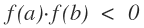
OK now call the midpoint of $a$ and $b$ point $c$.

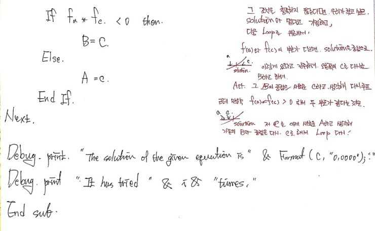
Now we make a call:

Is $f(a)f(c) < 0$?

Or is $f(c)f(b) < 0$?

Which one is it???

Oh, $f(a)f(c) < 0$, right? Cool — then call the midpoint of $a$ and $c$ our new $c'$.

And now, with $c'$ on the board,

we ask the same question again:

Is $f(a)f(c') < 0$??????

Or $f(c')f(c) < 0$???

Since it’s $f(c')f(c) < 0$,

the new $c''$ is

the midpoint of $c$ and $c'$…

You feel where this is going, right?

Just keep doing this on and ooooooooon

and eventually when you reach $c''''''''''''''''''''''''''''''''''''''''''''''''''''''''''''''''''\!\!\!\!\!\!\!\!\!\!\!\!\!\!\!\!\!\!\!\!\!\!\!\!\!\!\!\!....................''''''''$

even if it’s not exactly the solution we’re hunting for, won’t it be basically right on top of it?

That’s solution-finding via the bisection method!!!

Let’s actually use it.

Let’s find the root of this guy as practice.

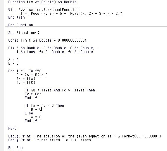
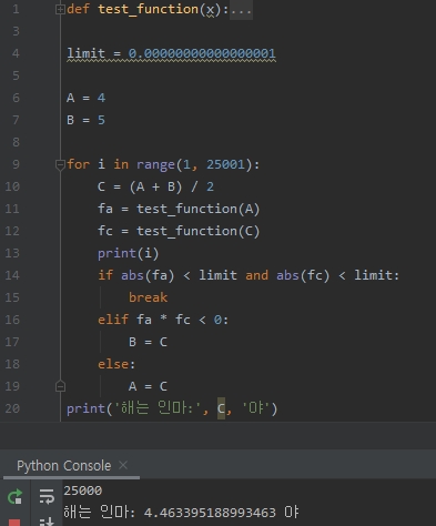
Python version

I also threw together a little video of it converging on the solution in Python

import matplotlib.pyplot as plt
import numpy as np
from matplotlib import font_manager, rc
font_name = font_manager.FontProperties(fname=r"c:\Windows\Fonts\malgun.ttf").get_name()
rc('font', family=font_name)
import matplotlib as mpl
mpl.rcParams['axes.unicode_minus'] = False

for i in range(1, 6):
    if i == 1:
        limit = 0.001
        A = -2
        B = 10
        x = np.linspace(-2, 7, 100)
        y = test_function(x)
        fig = plt.figure(figsize=(20, 10))
        ax = fig.add_subplot(111)
        fig = plt.plot(x, y)
        plt.axvline(x=0, color='k')
        plt.pause(1)
        plt.axhline(y=0, color='k')
        plt.pause(1)
        plt.scatter(A, 0, c='r', marker='*')
        plt.pause(1)
        ax.annotate('initial value', xy=(A, 0), xytext=(A+0.1, 1))
        plt.scatter(B, 0, c='r', marker='*')
        plt.pause(1)
        ax.annotate('initial value', xy=(B, 0), xytext=(B+0.1, 1))
    C = (A + B) / 2
    plt.scatter(C, 0, marker='*')
    ax.annotate('this time', xy=(C, 0), xytext=(C+1+i, 100),
                arrowprops=dict(facecolor='black', width=0.1, headlength=0.4, headwidth=1))
    plt.pause(1)
    fa = test_function(A)
    fc = test_function(C)
    if abs(fa) < limit and abs(fc) < limit:
        plt.scatter(C, 0, marker='*')
        ax.annotate('last time', xy=(C, 0), xytext=(C + 1, 110),
                    arrowprops=dict(facecolor='black', width=0.1, headlength=0.4, headwidth=1))
        plt.title('the solution, hey you jerk:', C, 'hey')
        break
    elif fa * fc < 0:
        B = C
    else:
        A = C

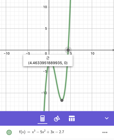
It comes out basically the same as the answer some app spits out!

(That app is running some algorithm too, lol.)

Just slapping a screenshot up and calling it a day feels kinda lazy though…

Back when I was studying this on my own,

I used to do it like this:

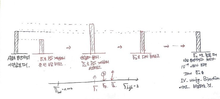
When you pick it apart that way,

you start to see the weak spots of the bisection method…

If the function is super flat near the root,

there’s a real chance it’ll declare some point “the solution” even though it’s still a noticeable distance away from the actual one.

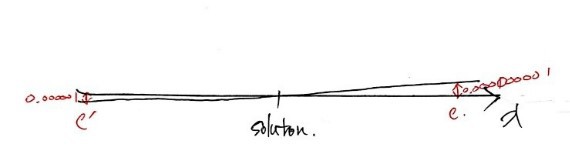
Like this kind of thing… right?????

Hold up!!!!!!!!! Wait,

why were we even learning the bisection method in the first place? — http://gdpresent.blog.me/220881927685

Right — it was specifically “to compute implied volatility.”

Implied Volatility — [Financial Engineering Programming I Studied #13]

In the previous post we looked at historical volatility. Why??? Because in the Black-Scholes model, “volatility…”

gdpresent.blog.me

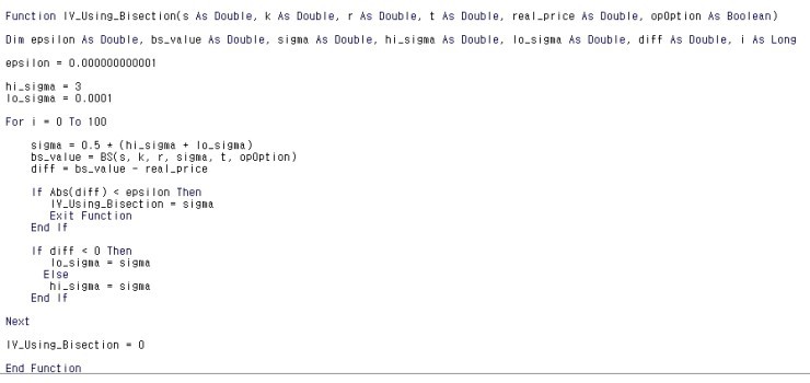
So this time, let’s actually use the bisection method idea

to compute the implied volatility.

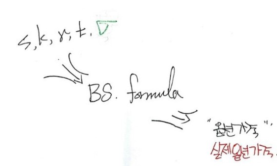
One more time: implied volatility is the $\sigma$ that makes the BS formula spit out exactly the market price!!!!!!!!!

For that, we need to feed in all 5 inputs

— $s, k, T, r, \sigma$ all at once! —

into a function that hands back the option price!

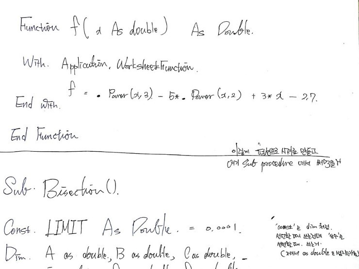
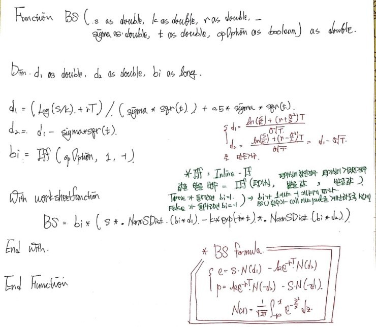
So let’s just write the whole thing out, starting with the function that does BS option pricing.

(let’s go let’s go)

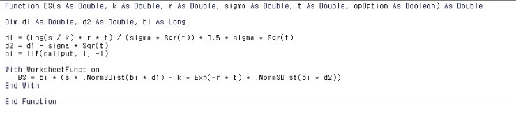
For the coding part, let me drop in a photo with some annotations on it,

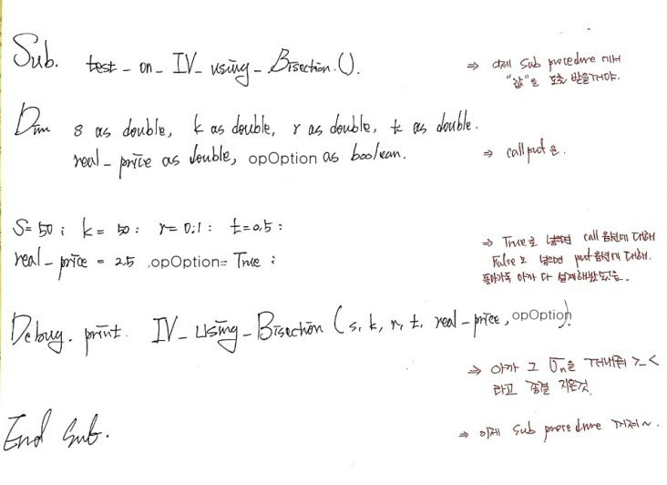
The code is so easy that it kinda explains itself,

but if I add a tiny bit more commentary —

Python version

import math
import scipy as sp
import scipy.stats
norm = sp.stats.norm(loc=0, scale=1)

def BS(S, k, r, sigma, t, opOption):
    d1 = (math.log(S / k) + r * t) / (sigma * math.sqrt(t)) + (0.5 * sigma * math.sqrt(t))
    d2 = d1 - (sigma * math.sqrt(t))
    if opOption == True:
        bi = 1
    else:
        bi = -1
    BS = bi * (S*norm.cdf(bi*d1) - k*math.exp(-r*t)*norm.cdf(bi*d2))
    return BS

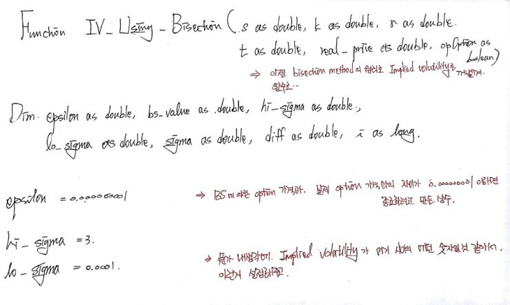
def IV_using_Bisection(S, k, r, t, real_price, opOption):
    epsilon = 0.0000000000000000000000000000001
    hi_sigma = 0.3
    lo_sigma = 0.0001
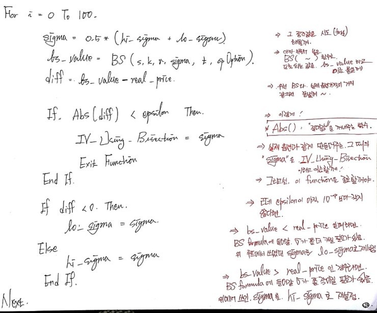
    for i in range(101):
        sigma = 0.5 * (hi_sigma + lo_sigma)
        bs_value = BS(S=S, k=k, r=r, sigma=sigma, t=t, opOption=opOption)
        diff = bs_value - real_price
        if abs(diff) < epsilon:
            IV_using_Bisection = sigma
            break
        else:
            pass
        if diff < 0:
            lo_sigma = sigma
        else:
            hi_sigma = sigma
    if abs(diff) < epsilon:
        IV_using_Bisection = IV_using_Bisection
    else:
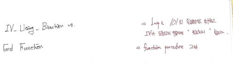
        IV_using_Bisection = 0
    return IV_using_Bisection

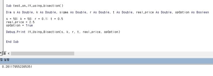
S=50; k=50; r=0.1; t=0.5
real_price = 2.5
opOption = False
IV_using_Bisection(S=S, k=k, r=r, t=t, real_price=real_price, opOption=opOption)

Now, this bisection method might come across as a bit of a brute.

Just going whack!!!!! — slap the midpoint in!!!!!!!! —

and yeah, sure, it does inch closer to the solution, juuust a little bit at a time…

So somebody clearly sat down and racked their brain over how to inch closer in a smarter way.

It’s called the weighted bisection method,

and… yeah, looks like a way to cut down on the number of iterations a bit.

Let me just explain it real quick with a picture and move on.

A second ago it was, “no questions, just gimme the midpoint!!!!” —

now, instead of jumping to the midpoint of $a$ and $b$,

we look at the function values at $a$ and $b$, draw the straight line between those two points, and then —

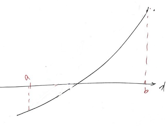
— first off, we want to head over to where the solution is, so how do we get closer? Well —

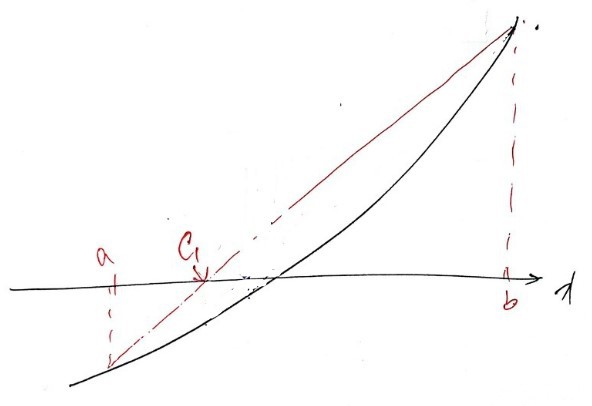
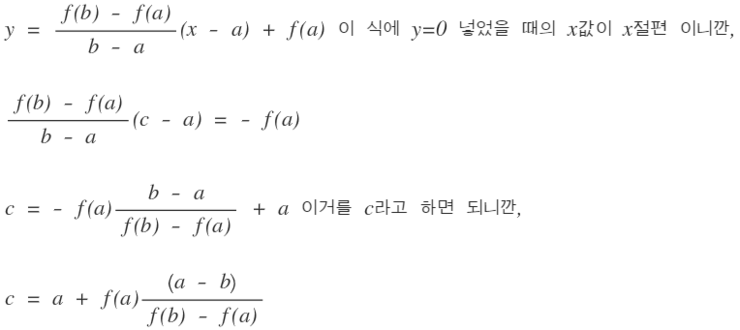
— we draw the line equation between the two function values,

and we call the $x$-intercept of that line $c$ again.

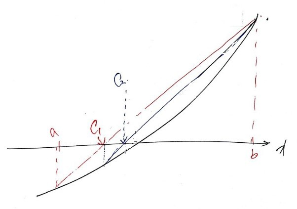
Then at that $c$, we draw another line between the two new points,

and we call the $x$-intercept of that line $c$ again. heh heh heh heh

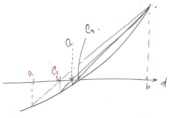
OK now you feel how it closes in on the solution, right?

Oh — but before, $c = (a+b)/2$ which was easy,

how do we write down the next $c$ this time??????!?!?!?

The line connecting $(a, f(a))$ and $(b, f(b))$ is

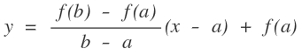
— that’s the line equation, and

So using that, let’s run the weighted bisection method on

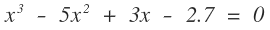
— the same equation we were playing the solution-finding game with above.

The function bit we can just reuse from before,

so we only need to write the sub-procedure. heh

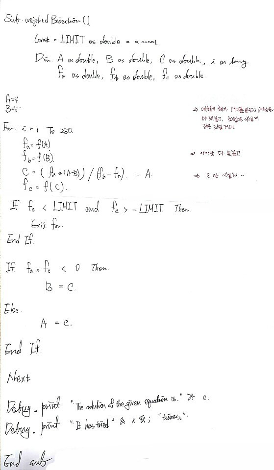
Python version

def f(x):
    return x ** 3 - 5 * x ** 2 + 3 * x - 2.7

A = 4
B = 5
limit = 0.000000000000000001
for i in range(251):
    fa = f(A)
    fb = f(B)
    c = (fa * (A - B)) / (fb - fa) + A
    fc = f(c)
    if (fc < limit) & (fc < -limit):
        break
    else:
        pass
    if fa * fc < 0:
        B = c
    else:
        A = c
print('The solution of the given equation is ', c)

Originally written in Korean on my Naver blog (2016-12). Translated to English for gdpark.blog.