Newton-Raphson Method

So as I mentioned last time, I’m trying to find implied volatility, and I already took one swing at it with the bisection method. Now let’s go again — this time with Newton-Raphson.

But before we touch any code, let’s figure out how Newton-Raphson actually sneaks up on a solution. What’s the algorithm? How does it cook up an approximation? Let’s walk through it.

How Newton-Raphson works

Here’s the idea.

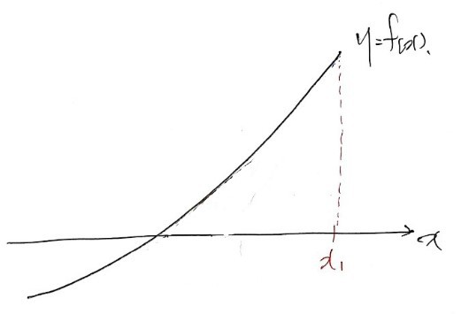
Step one: pick some $x_1$ and plug it into the function.

(In practice you wouldn’t pick just anything. You’d pick something as close to the solution as you can guess. For efficiency, for economy, for not wasting your life, etc., etc.~)

Plug it in — and oh god, $f(x_1)$ is huge. Way off. So $x_1$ is clearly not our solution.

So from the point $(x_1, f(x_1))$, draw the tangent line. Take the x-intercept of that tangent line and call it $x_2$. Plug $x_2$ back into $f(x)$. Is $f(x_2)$ still ridiculously far from 0? Or are we getting close?

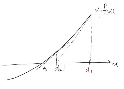
Still off? Cool. Draw the tangent line at $(x_2, f(x_2))$, take its x-intercept, call it $x_3$, judge again, and keep going~~~~~~~~~~~~~~~ and going~~~~~~~~~~~~~~~ and going~~~~~~~~~~~~

Done~

Honestly mind-blowing. And honestly — kind of insane that someone thought of this in the first place.

OK now write it down

So we kinda get the vibe. Now we have to turn it into formulas, because the computer doesn’t speak English (or Korean, or whatever), it speaks math.

The computer is basically asking us:

“hey jerk —

to

what’s the rule? how do I get from one to the other?????”

OK. The tangent line at the point $(x_n, f(x_n))$ is:

Undeniable. Slope is $f'(x_n)$, line passes through

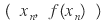
— that’s literally just point-slope form.

And $x_{n+1}$ is the $x$ where this tangent line hits $y = 0$. Set $y = 0$, solve for $x$, and:

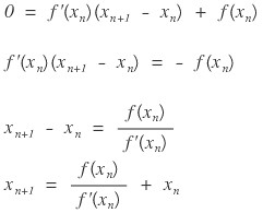
Boom. That’s the recurrence.

Easy!!!!!!!!!!!!!!!!!!!!!!!!

Let’s play

Let’s use this on our usual suspect:

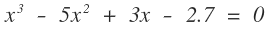
(Why is it ALWAYS this one???????????? Because I already wrote the function for it last time^^ heh heh heh if you want a different example, you write it^^^^^^^^^^^^^^^^^^^^)

Ugh, but… we need a new function. Specifically, we need one for the derivative.

Ughhhhhh ;; ;; ;; ;;

OK OK OK OK. The derivative of that thing is something a 10th grader can do in their sleep. Bang it out. Then on to the code.

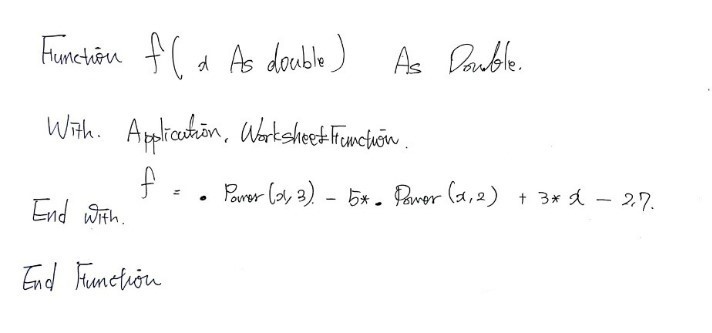
This one’s the function we used for bisection last time~~

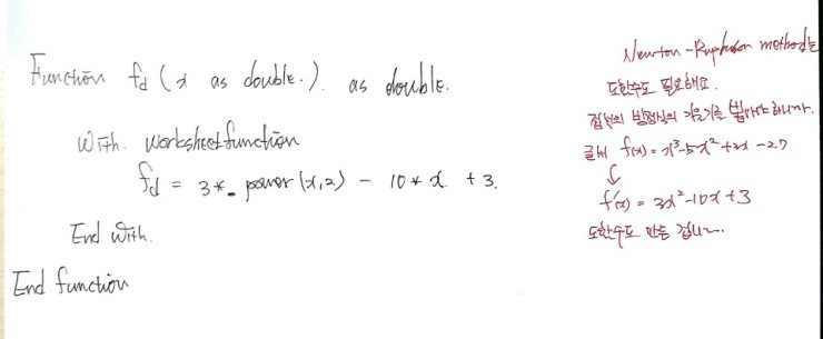
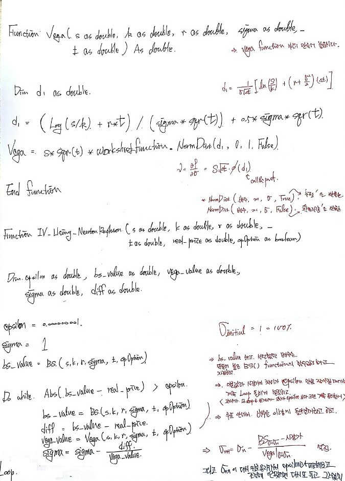
This one is just the derivative of it — differentiated by hand and dropped into a function.

Easy, right?

We literally just used the principle we walked through above:

That’s it. heh.

Now the actual implied vol part

OK, now using Newton-Raphson, let’s go extract the implied volatility of an option.

Wait hold on. Newton-Raphson needs $f(x)$ AND $f'(x)$, right? So before we sprint ahead, there’s something worth thinking about.

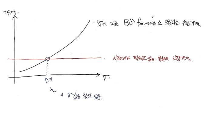
I drew option price as an increasing function of $\sigma$ — is that actually right?

Yeah, it’s right. Options have no downside risk, so their value goes up as volatility goes up. I mentioned this somewhere before — over here, I think.

Options [ Financial Derivatives I Studied #10 ]

I hear the derivatives class I’m taking is split into before and after the midterm. As in: No Options, and Options…..

gdpresent.blog.me

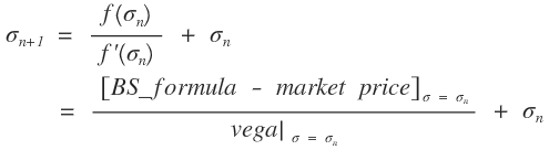
Anyway. What we want is the $\sigma$ at the intersection point over there. That is:

Let’s call the left side $f(\sigma)$:

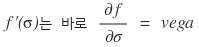
We want $f(\sigma) = 0$. And the derivative we need for Newton-Raphson is $f'(\sigma)$:

The market price is a constant, so its derivative with respect to $\sigma$ is 0.

So what I’m trying to say is —

THAT is the thing!!!!

The derivative we need for Newton-Raphson is vega!!!

Eek!!!! AND!!!! We’ve already learned about vega before!!!!

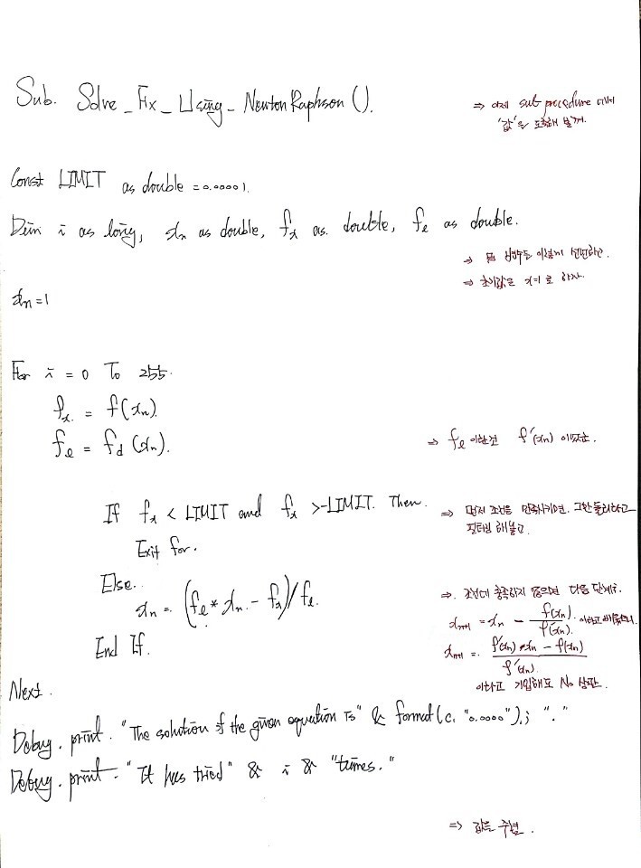
OK so. Now in our $y = f(x)$ Newton-Raphson recurrence,

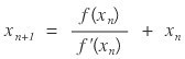
the relationship between these — how do we use it here~~

Based on everything above, we can just write it like this:

Let’s code it

Time to actually code it up and find the implied volatility.

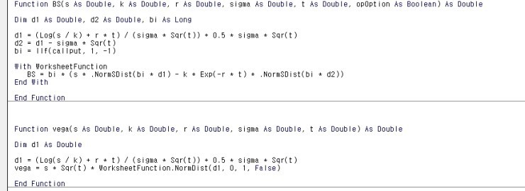
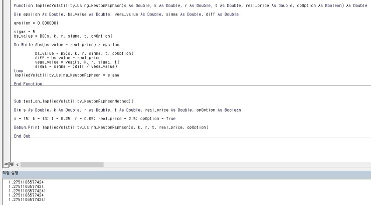
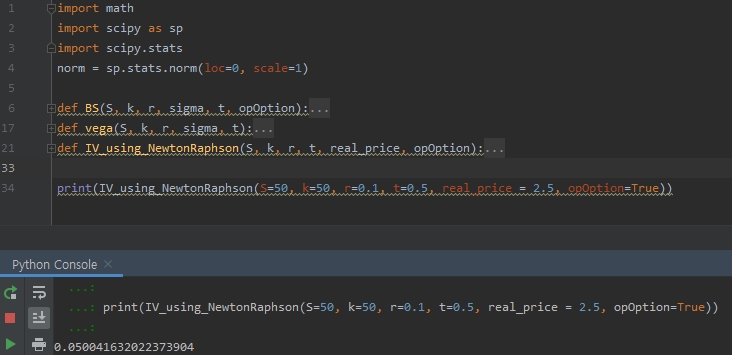
In the output you’ll see a bunch of implied volatility values — that’s because I tried it with a bunch of different initial volatility values. They all converge to the same number.

But — you might be feeling a little uneasy about that initial volatility, right? And if you plug in something absurdly large there, vega comes out as 0, and the code just dies.

So picking the initial volatility appropriately turns out to matter. Apparently there’s a lot of research on this. But it’s not what I’m focused on right now, so I’ll skip it. I just plugged in some arbitrary value. (Honestly, just using the historical volatility is probably fine too.)

Anyway, let’s keep moving heh heh heh heh

Python version!

import math
import scipy as sp
import scipy.stats

norm = sp.stats.norm(loc=0, scale=1)

def BS(S, k, r, sigma, t, opOption):
    d1 = (math.log(S / k) + r * t) / (sigma * math.sqrt(t)) + 0.5 * sigma * math.sqrt(t)
    d2 = d1 - (sigma * math.sqrt(t))
    if opOption == True:
        bi = 1
    else:
        bi = -1
    BS = bi * (S*norm.cdf(bi*d1) - k*math.exp(-r*t)*norm.cdf(bi*d2))
    return BS

def vega(S, k, r, sigma, t):
    d1 = (math.log(S / k) + (r * t)) / (sigma * math.sqrt(t)) + 0.5 * sigma * math.sqrt(t)
    vega = S*math.sqrt(t) + norm.pdf(d1)
    return vega

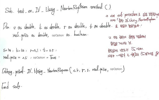
def IV_using_NewtonRaphson(S, k, r, t, real_price, opOption):
    epsilon = 0.0000000000001
    sigma = 5
    bs_value = BS(S=S, k=k, r=r, sigma=sigma, t=t, opOption=opOption)
    while abs(bs_value - real_price) > epsilon:
        bs_value = BS(S=S, k=k, r=r, sigma=sigma, t=t, opOption=opOption)
        diff = real_price - bs_value
        vega_value = vega(S=S, k=k, r=r, sigma=sigma, t=t)
        sigma = sigma + (diff/vega_value)
    return sigma

S=50; k=50; r=0.1; t=0.5
real_price = 2.5
opOption=True
IV_using_NewtonRaphson(S=S, k=k, r=r, t=t, real_price=real_price, opOption=opOption)

Originally written in Korean on my Naver blog (2016-12). Translated to English for gdpark.blog.