Differentiation Fundamentals for Finite Difference Methods

Quick recap of where we’ve been so far. We learned option pricing via Black-Scholes in a totally half-assed way, and one of the 6 assumptions baked into that model was constant volatility.

So — what number do we plug in for that “constant”? Reasonable question. That got us into historical volatility, which is simple, and honestly… not unreasonable? “The present is just history on repeat” and all that. But it also feels like it can’t really capture the options that are actually trading out there in the wild.

So people went, “OK fine — let’s just back out the volatility that real-world option prices are implying.” And boom, implied volatility.

But the BS formula isn’t exactly the kind of expression you can flip inside out and pull a clean inverse from. So instead of grinding through it by hand, we hand it to a computer. And then — OK, how do we make the computer do it? — and that’s where Bisection, Weighted Bisection, and Newton-Raphson came in.

(After implied vol, the proper next step would be volatility models — EWMA, ARCH, GARCH(1,1), the whole crew. But this is a financial engineering programming class, so we’re skipping them.)

(I’ll do a separate post on those guys later.)

OK. Stepping away from volatility for now. Let’s go back to where we started — back to the Black-Scholes PDE, the one that won the Nobel Prize in Economics.

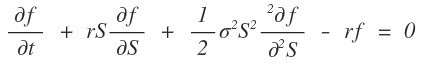
Here $f$ is the value of a portfolio, but for our purposes we’re treating it as the value of an option.

And notice — that “value” function is being partial-differentiated with respect to maturity $t$, and with respect to the underlying $S$, and so on. So yeah, we can comfortably think of $f$ as a function of two variables: $t$ and $S$.

Right. So the goal, starting from this chapter, is:

Find $f(t, S)$!!!!!!

Except… that PDE? You can’t crack it open.

Can’t be solved??????? What does that even mean????????

Well, in this world, there genuinely do exist equations that can’t be solved. In physics the textbook example is probably the Schrödinger equation.

(OK, for the hydrogen atom you can pull some tricks and actually solve it, but the moment you hit helium — 2 protons or more — totally hopeless…)

Which is exactly why a whole arsenal of tricks got invented — WKB, perturbation theory, all of that.

And the heat equation is the same vibe — it’s a PDE in time and position, and a lot of machinery exists purely to wrestle that thing into something solvable.

Same context here. The Black-Scholes PDE is, well… troublesome. There’s no clean analytic solution to pull out.

So we cheat. With a numerical trick called FDM (Finite Difference Method).

Now — before we touch FDM, we need to sharpen our concept of differentiation just a tiny bit. I’m not a math tutor so this might be a little rough, but let’s run through it once.

When you’re staring at some function, there’s a bunch of stuff you want to get a handle on, and one of the most important — maybe the most important — is the slope.

If $f(t)$ is, say, your “grades” as a function of time $t$, then sure — the actual grade value $f(t)$ matters. But $df(t)/dt$ — the rate of change of your grade per unit time — that’s also pretty critical info if you’re trying to actually grasp what’s going on.

So the slope ends up being a big deal in lots of situations… yeah, yeah, yeah.

Now — slope between two points is fine, but what’s really meaningful is the derivative — the instantaneous slope at a point.

The instantaneous slope at some point $x = a$ — once you’ve learned $\lim$ in high school and you wield that limit concept —

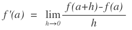
— gets defined like this, right??? The reason I’m dragging us through this baby definition again is because there’s a question worth raising: “does the derivative at $x = a$ have to be that one?????”

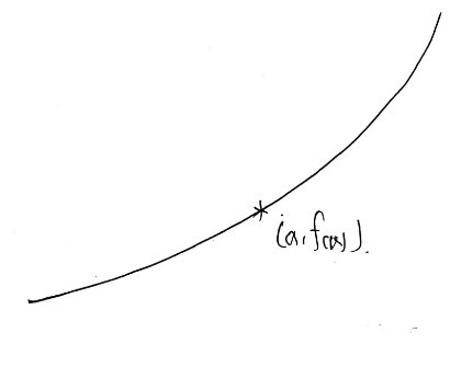
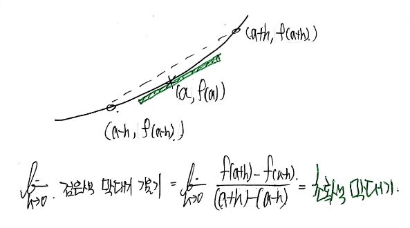
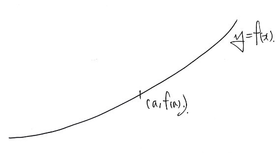
OK so we want the derivative at the point $(a, f(a))$. In the standard story, you grab a point $h$ to the right —

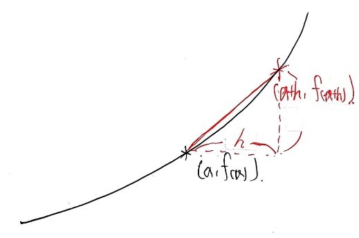
— and look at the slope between $(a+h, f(a+h))$ and $(a, f(a))$, which gives you

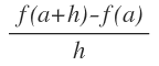
— and that’s the slope of the red line, and then you take $h \to 0$ —

— and there’s your derivative. Classic high-school flow.

But — like I said — does it have to be that?

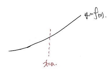
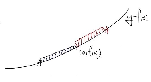
What if instead I do this:

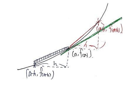
Define the blue point as $(a-h, f(a-h))$, take the slope of the blue line —

— this one — and then send $h \to 0$ —

— and call it a day. Honestly? Nothing wrong with that either.

(Strictly speaking, both are valid — the difference is whether it’s the right-hand limit or left-hand limit of the derivative.)

The point I’m hammering: differentiating at $x = a$ — you can do it this way, or you can do it that way. Heh.

Aaaand… it doesn’t even stop there.

“Hey~~~ you two, I’m just gonna combine both of your methods and define it like this~~~ ^^^^”

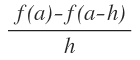
And then if someone draws this picture and writes the expression below like this:

That is also a perfectly valid derivative at $x = a$… (cry)(cry)(cry)(cry)(cry)

All three are valid… (cry)(cry)(cry)(cry)(cry)

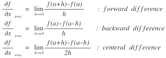
So actually there are three ways to differentiate.

(High school teaches this same way too, by the way.)

But — unfortunately — in numerical analysis, there is no way to actually… do that $h \to 0$ thing from math class.

So instead, we approximate the derivative.

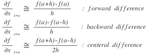
Approximation looks like this…

Ah, but that’s approximating the derivative at a point. If we shift to talking about the derivative function:

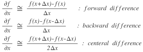
Writing it like this is fine, right? Of course $\Delta x$ has to be sufficiently small.

Ah but — the whole reason we pulled out the differentiation concept up there —

— was to approximate the partial derivative of $f(x,t)$ in this Black-Scholes PDE with respect to $t$ at each position, the partial with respect to $S$, the second partial with respect to $S$, all that stuff, right???

So:

Writing it in this scrappy way will do the trick.

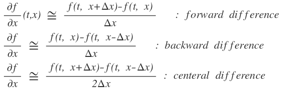
The variable $t$ shows up, but since it’s a partial derivative, $t$ is being held fixed in the formula.

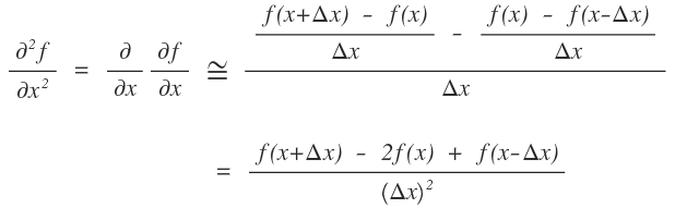
But — as you can see in the BS PDE — there’s also a second partial with respect to $S$. We need to express that too.

Good news: for the second derivative, there aren’t three options.

Why? Because if you differentiate forward twice, you’ve drifted away from $x=a$ — hard to call that “the second derivative at $x=a$” anymore. Same problem going backward twice.

So, the second derivative is — the measure of how much does the slope change at $x = a$ —

— the instantaneous slope at $x = a$ goes from the slope of the blue line (backward) to the slope of the red line (forward).

That feels like the natural way to phrase it.

Therefore,

OK — this approximation-of-derivatives detour ran way longer than I planned. I was going to push into Explicit FDM in this post, but……

Ahhh……… pushing it to the next post.

Starting from the next post, we’ll get into Explicit FDM properly.

Originally written in Korean on my Naver blog (2016-12). Translated to English for gdpark.blog.