Picking up right where we left off last time.

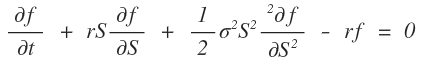
So in the Black-Scholes PDE,

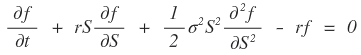
…we’ve now finished prepping all the “approximation formulas” for the 1st-order and 2nd-order derivative terms sitting in there.

OK then, quick reminder of what we’re actually trying to do.

We can’t find an analytic solution for $f(t,S)$ that satisfies this PDE.

Why? Because that PDE is, well, one of those PDEs you just can’t solve in closed form.

(Kind of like the Schrödinger equation in the nasty cases, maybe…?)

But we still want to know $f(t,S)$. That’s the whole problem. T_T T_T T_T T_T

So what sneaky trick did we cook up?

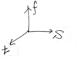
Since we can’t draw $f(t,S)$ as a smooth function across the whole space like this,

let’s just mark every single function value at every single $(t,S)$ point one by one, like in that picture!!!!!! That’s the move.

Now, the reason this is even possible —

it’s because options have this peculiar property —

specifically, the property that

the value of the option at maturity is $S-k$,

and because options have that going for them,

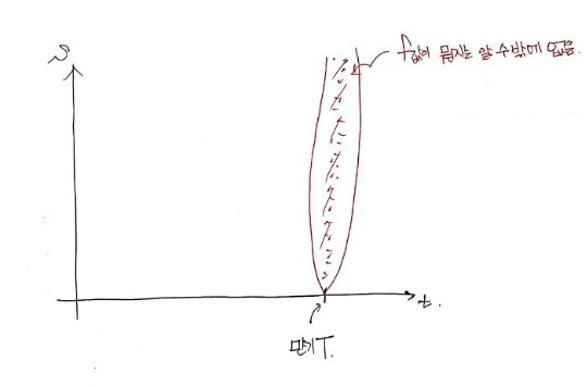
at least along here, we can flat-out say $f = S - k$.

And also,

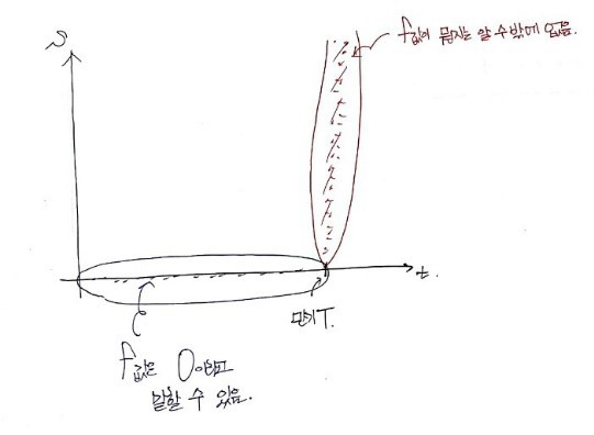
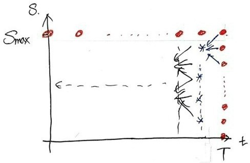
when $S=0$ like this, we can also say the option value is 0.

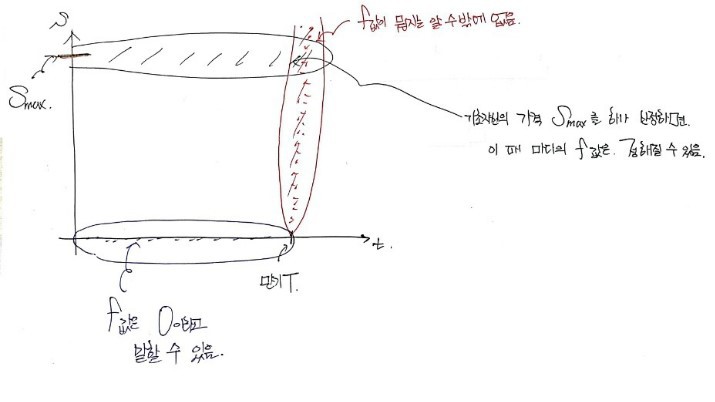
Also! Let’s set some upper bound on the underlying price $S$.

(There’s no way the underlying price actually shoots off to infinity, riiight????????? So we pick some $S_{\max}$ that’s “high enough” and call it good.)

So once we fix one max price for $S$,

at $S_{\max}$, for all $t$,

since $S$ is always going to be way bigger than $k$ there,

the option value $f$ at each $t$ is

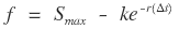
We can just say that!!!!!

So putting it all together,

out of the giant pile of values we have to figure out,

it turns out we already know everything along that “boundary” — the upside-down ㄷ-shaped frame around the region.

OK so then, how do we find the inside?

Finding it for continuous $S$ and $t$? Impossible. (If we could do that, we’d basically be solving the PDE analytically. Which, no.)

So instead of finding it for continuously varying $S$ and $t$, let’s find it “sparsely” first!!!!!

We’re going to slice up the coordinate plane.

Cut $S$ into $n$ equal pieces, cut $T$ into $m$ equal pieces.

Same-size chunks. Equal divisions.

And since the spacings are uniform,

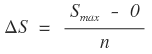
the spacing $\Delta S$ along the $S$-axis is

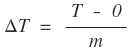
And on the $t$-axis, since we’re cutting from now up to maturity $T$ into $m$ chunks,

OK so now, how do we want to express the option price $f$?

When we’re at

we’re not going to ask “what’s the option value at”

Instead,

we go $i$ steps of $\Delta T$ in the $t$ direction, and

$j$ steps of $\Delta S$ in the $S$ direction,

and we ask for the option value at that gridpoint:

— that’s the question we’ll be asking from now on.

(Don’t get spooked when $f_{i,j}$ shows up, heh heh heh heh.)

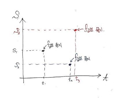
Ahhhhh OK so if we look at this whole setup as a picture,

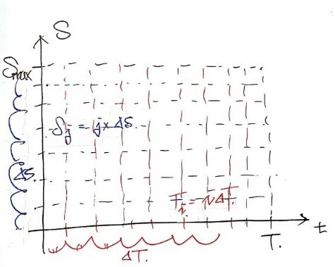
what we want to do is figure out every single

sitting at every dotted-line intersection.

But!!!!!

Don’t forget — for all the

sitting on that upside-down-ㄷ boundary, we already know the answer~~!!!

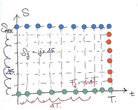
Those dots right there. heh heh heh — kya kya kya.

Alright. Now let me actually get into Explicit FDM.

In “Financial Engineering Programming I’m Studying,” among the FDM family,

we’ll cover 3 flavors of FDM.

Explicit FDM, Implicit FDM, Crank-Nicolson FDM —

those 3,

and Explicit FDM is the very first one!!!!!!!!

First up, let’s get the dictionary definition out of the way.

Finite Difference Method: a method for numerically analyzing a PDE by approximating it as a difference equation.

Or: a method for numerically getting the solution by carving the space governed by the PDE into a small grid.

That’s the gist. From here on we get into the actual Explicit FDM procedure for solving the PDE —

and as for why it’s called “Explicit,”

well, in like… 60 seconds??? you’ll just automatically get it.

First,

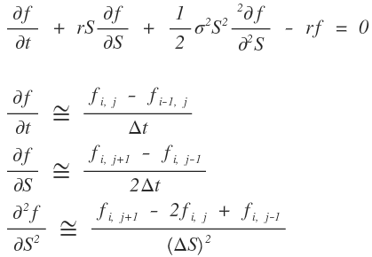
we’re going to “approximate” all the partial derivative terms in our annoying function.

How?

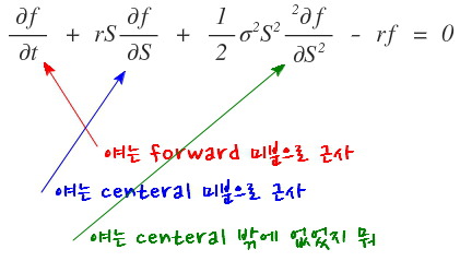
Like this — we substitute each term in this exact way.

“Why backward for $t$ and central for $S$??????????????????????????????” you ask?

Answer: so the whole thing comes out “Explicit”!!!

That’s all I can tell you for now….

What????????????????????

About 40 seconds left. In 40 seconds you’ll just see it. ^^ heh heh

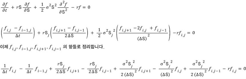
OK so if we sub each of those into the PDE,

(real talk, typing this out in the equation editor is an absolutely insane act of self-harm, but let me try once)

I’ll only get that far in the equation editor — beyond this point my handwriting is gonna serve us better.

(“My handwriting is gonna serve us better.” = “I’m too lazy to keep typing this in the equation editor.”) Synonyms.

Honestly when am I ever gonna finish typing all that, lol lol lol lol lol lol lol lol lol lol lol

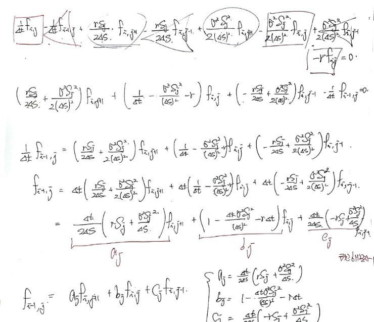
Yay~~~~~ all cleaned up~~~~~~~~~~~~~~~~~~

When we “approximate” the PDE in this form,

we can find every single $f_{i,j}$.

Let’s see why.

If we just look at that tidied-up equation as

it’s like this!!!!

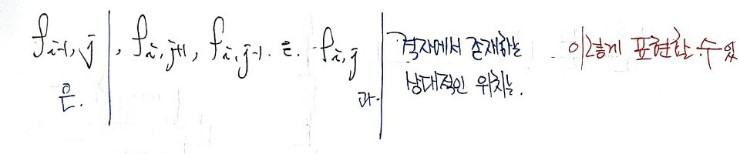
Each one lives at that position in the grid!!!!!!!

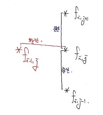
Aha!!! So the option value at an arbitrary position $i$ in $t$ and $j$ in $S$

is the sum — with appropriate coefficients — of three values sitting at $j+1$, $j$, $j-1$ at the $i+1$ position in $t$!!

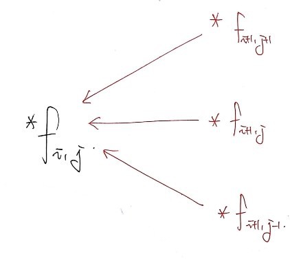
What I’m saying is, $f_{i,j}$ is just the right blend of those 3 option values $f_{i+1,j+1}$, $f_{i+1,j}$, $f_{i+1,j-1}$ sitting over there!!!!

Hold on though — don’t we also not know those 3 values??!?!?!?!

Nah… we know the boundary.

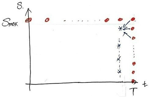
Because we know the boundary, this process lets us find every $f$ value one step back in $t$. ha.

Then using those values we just found,

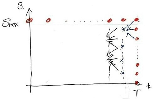
we step back one more.

Same logic, all the way back. Trivial from here, right??!?!?

OK so — getting a feel for why this FDM is called Explicit FDM in the first place????

In econ there’s this term, “explicit cost.”

It’s the cost measured exactly as it visibly shows up.

That’s “explicit cost” in English,

and in the same spirit, I think this FDM got its name because $f_{i,j}$ is determined explicitly from the visible “$f_{\text{maturity}, j}$ values.”

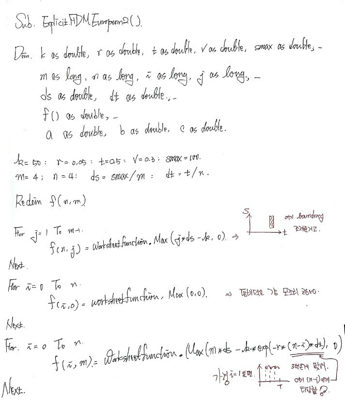
Alright, let’s actually code this thing up.

I’ll do it for a European Call.

Since it’s a European call, the payoff condition at $t = \text{maturity}(T)$ is

$\max(\Delta S \cdot j - k,\ 0)$, right???? OK let’s go.

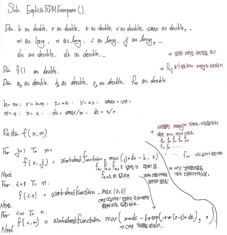
I actually went and coded this myself!!!!!!!!!!!!!

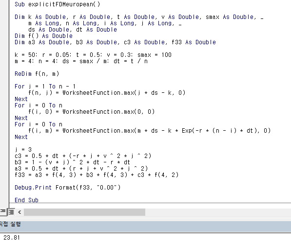
I mentioned this above when we were doing concepts, but

when you plug in the boundary conditions in the code,

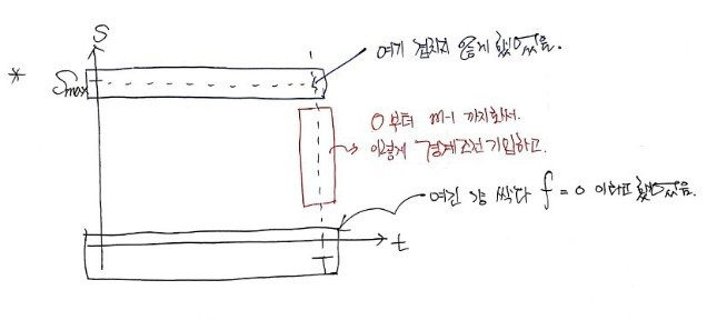
notice how I plug them in like this,

and

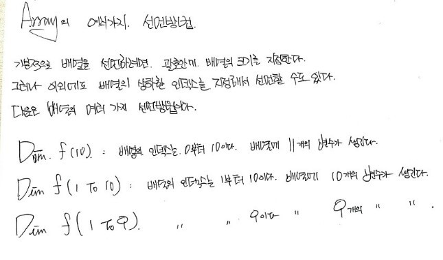
I know I covered it once before way back, but

I’ll briefly redo array declarations one more time.

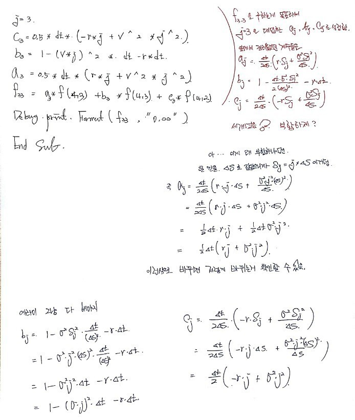
OK so now, instead of just one value like $f_{3,3}$,

let’s set the code up so that we get out every $f_{i,j}$ across the whole grid.

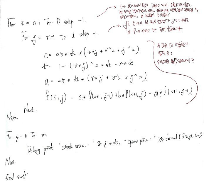
I’ll code this one up too!!!!!

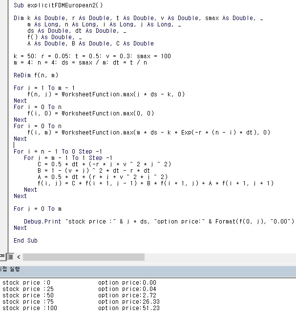
Surprisingly simple, right??!?!?!?!

Surprisingly easy.

But — the

Implicit FDM and Crank-Nicolson FDM coming up next are not gonna be a pushover.

hihihihihihihihihi alright see you next time heh

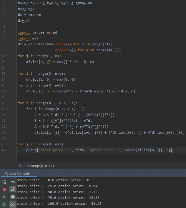
python version

k=50; r=0.05; t=0.5; v=0.3; smax=100
m=4; n=4
ds = smax/m
dt=t/n
import pandas as pd
import math
df = pd.DataFrame(index=[x for x in range(n+1)],
                  columns=[y for y in range(m+1)])
for j in range(1, m):
    df.loc[n, j] = max(j * ds - k, 0)
for i in range(0, n+1):
    df.loc[i, 0] = max(0, 0)
for i in range(0, n+1):
    df.loc[i, m] = max(m*ds - k*math.exp(-r*(n-i)*dt), 0)
for i in range(n-1, 0-1, -1):
    for j in range(m-1, 1-1, -1):
        C = 0.5 * dt * (-r * j + (v**2)*(j**2))
        B = 1 - ((v*j)**2)*dt - r*dt
        A = 0.5 * dt * (r*j + (v**2)*(j**2))
        df.loc[i, j] = C*df.loc[i+1, j-1] + B*df.loc[i+1, j] + A*df.loc[i+1, j+1]
for j in range(0, m+1):
    print('stock price : ', j*ds, "option price: ", round(df.loc[0, j], 2))

Originally written in Korean on my Naver blog (2016-12). Translated to English for gdpark.blog.