Implicit Finite Difference Method (FDM)

OK let’s just keep going.

This time: Implicit FDM.

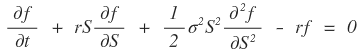
Last time, when we approximated the Black-Scholes PDE,

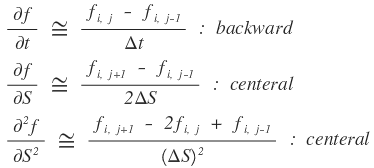
this version — that was Explicit FDM.

So now, this Implicit FDM thing — how does it approximate? Same idea, except instead of doing a backward difference in $t$, we do a forward difference.

That is:

we approximate

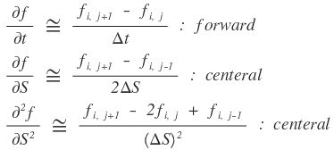
like this!!!!!!

So why does flipping that one direction make it “implicit”?!?!

Honestly — the reason it’s called Implicit only really shows up after you plug everything in and grind through the algebra. Just plug it in. Organize. You’ll see.

If that explanation isn’t doing it for you — same. Just plug it in and shuffle terms!! heh heh heh

OK, brace yourself. I’m gonna type the whole thing into the equation editor. I’m going to lose my mind doing this!!!!!!

$$\frac{\partial f}{\partial t} + rS\frac{\partial f}{\partial S} + \frac{1}{2}\sigma^{2}S^{2}\frac{\partial^{2}f}{\partial S^{2}} - rf = 0 \\ S = S_{j} = j\cdot\Delta S\\ t = t_{i} = i\cdot\Delta t \quad \text{approximation at} \\ \left|\frac{\partial f}{\partial t}\right|_{\substack{t=t_{i}\\S=S_{j}}} + rS_{j}\left|\frac{\partial f}{\partial S}\right|_{\substack{t=t_{i}\\S=S_{j}}} + \frac{1}{2}\sigma^{2}S_{j}^{2}\left|\frac{\partial^{2}f}{\partial S^{2}}\right|_{\substack{t=t_{i}\\S=S_{j}}} - r\left|f\right|_{\substack{t=t_{i}\\S=S_{j}}} = 0$$$$\left(\frac{f_{i+1,j} - f_{i,j}}{\Delta t}\right) + rS_{j}\left(\frac{f_{i,j+1} - f_{i,j-1}}{2\Delta S}\right) + \frac{1}{2}\sigma^{2}S_{j}^{2}\left(\frac{f_{i,j+1} - 2f_{i,j} + f_{i,j-1}}{(\Delta S)^{2}}\right) - rf_{i,j} = 0 \\ \frac{1}{\Delta t}f_{i+1,j} - \frac{1}{\Delta t}f_{i,j} + \frac{rS_{j}}{2\Delta S}f_{i,j+1} - \frac{rS_{j}}{2\Delta S}f_{i,j-1} + \frac{\sigma^{2}S_{j}^{2}}{2(\Delta S)^{2}}f_{i,j+1} - \frac{\sigma^{2}S_{j}^{2}}{(\Delta S)^{2}}f_{i,j} + \frac{\sigma^{2}S_{j}^{2}}{2(\Delta S)^{2}}f_{i,j-1} - rf_{i,j} = 0 \\ \frac{1}{\Delta t}f_{i+1,j} + \left(\frac{rS_{j}}{2\Delta S} + \frac{\sigma^{2}S_{j}^{2}}{2(\Delta S)^{2}}\right)f_{i,j+1} + \left(-\frac{1}{\Delta t} - r - \frac{\sigma^{2}S_{j}^{2}}{(\Delta S)^{2}}\right)f_{i,j} + \left(-\frac{rS_{j}}{2\Delta S} + \frac{\sigma^{2}S_{j}^{2}}{2(\Delta S)^{2}}\right)f_{i,j-1} = 0$$$$\frac{1}{\Delta t}f_{i+1,j} = -\left(\frac{rS_{j}}{2\Delta S} + \frac{\sigma^{2}S_{j}^{2}}{2(\Delta S)^{2}}\right)f_{i,j+1} + \left(\frac{1}{\Delta t} + r + \frac{\sigma^{2}S_{j}^{2}}{(\Delta S)^{2}}\right)f_{i,j} + \left(\frac{rS_{j}}{2\Delta S} - \frac{\sigma^{2}S_{j}^{2}}{2(\Delta S)^{2}}\right)f_{i,j-1}\\ \frac{1}{\Delta t}f_{i+1,j} = -\frac{1}{2\Delta S}\left(rS_{j} + \frac{\sigma^{2}S_{j}^{2}}{\Delta S}\right)f_{i,j+1} + \left(\frac{1}{\Delta t} + r + \frac{\sigma^{2}S_{j}^{2}}{(\Delta S)^{2}}\right)f_{i,j} + \frac{1}{2\Delta S}\left(rS_{j} - \frac{\sigma^{2}S_{j}^{2}}{\Delta S}\right)f_{i,j-1}\\ f_{i+1,j} = -\frac{\Delta t}{2\Delta S}\left(rS_{j} + \frac{\sigma^{2}S_{j}^{2}}{\Delta S}\right)f_{i,j+1} + \left(1 + r\Delta t + \frac{\Delta t\sigma^{2}S_{j}^{2}}{(\Delta S)^{2}}\right)f_{i,j} + \frac{\Delta t}{2\Delta S}\left(rS_{j} - \frac{\sigma^{2}S_{j}^{2}}{\Delta S}\right)f_{i,j-1}$$$$f_{i+1,j} = -\frac{\Delta t}{2\Delta S}\left(rS_{j} + \frac{\sigma^{2}S_{j}^{2}}{\Delta S}\right)f_{i,j+1} + \left(1 + r\Delta t + \frac{\Delta t\sigma^{2}S_{j}^{2}}{(\Delta S)^{2}}\right)f_{i,j} + \frac{\Delta t}{2\Delta S}\left(rS_{j} - \frac{\sigma^{2}S_{j}^{2}}{\Delta S}\right)f_{i,j-1} \\ \text{Let's call each of the coefficient terms } a_{j},\ b_{j},\ c_{j}\\ f_{i+1,j} = a_{j}\cdot f_{i,j+1} + b_{j}\cdot f_{i,j} + c_{j}\cdot f_{i,j-1} \\ \begin{cases}{a_{j} = -\frac{\Delta t}{2\Delta S}\left(rS_{j} + \frac{\sigma^{2}S_{j}^{2}}{\Delta S}\right)}\\{b_{j} = \left(1 + r\Delta t + \frac{\Delta t\sigma^{2}S_{j}^{2}}{(\Delta S)^{2}}\right)}\\{c_{j} = -\frac{\Delta t}{2\Delta S}\left(-rS_{j} + \frac{\sigma^{2}S_{j}^{2}}{\Delta S}\right)}\end{cases}$$$$\text{Finally, since we cut at } S_{j} = j\cdot\Delta S\text{, plugging that in and organizing just once} \\ \begin{cases}{a_{j} = -\frac{\Delta t}{2\Delta S}\left(rS_{j} + \frac{\sigma^{2}S_{j}^{2}}{\Delta S}\right) = -\frac{\Delta t}{2}\left(rj + \sigma^{2}j^{2}\right)}\\{b_{j} = \left(1 + r\Delta t + \frac{\Delta t\sigma^{2}S_{j}^{2}}{(\Delta S)^{2}}\right) = 1 + r\Delta t + \Delta t\sigma^{2}j^{2}}\\{c_{j} = -\frac{\Delta t}{2\Delta S}\left(-rS_{j} + \frac{\sigma^{2}S_{j}^{2}}{\Delta S}\right) = -\frac{\Delta t}{2}\left(-rj + \sigma^{2}j^{2}\right)}\end{cases}$$

…I cannot believe I just typed all of that. I’m losing it.

Anyway!!!!

Here’s what Implicit FDM actually gives us:

$$f_{i+1,j} = a_{j}\cdot f_{i,j+1} + b_{j}\cdot f_{i,j} + c_{j}\cdot f_{i,j-1}$$

or equivalently — let me just shift indices —

$$f_{i,j} = a_{j}\cdot f_{i-1,j+1} + b_{j}\cdot f_{i-1,j} + c_{j}\cdot f_{i-1,j-1}$$

OK so what is this equation actually saying~~~

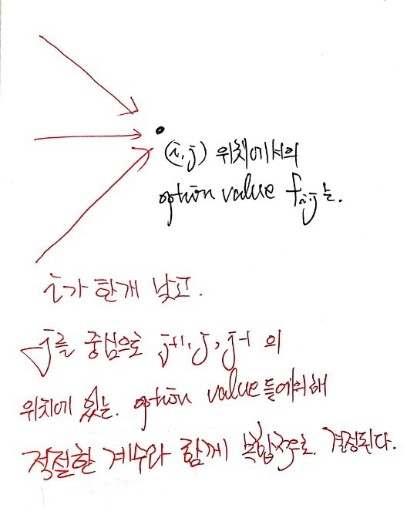
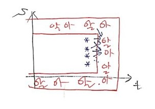
Visually, it’s saying this. heh heh heh

But hold on.

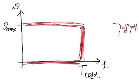
The values we know — the knowns — they’re over here.

And so:

In Explicit FDM, we got to march across and fill in the unknown middle guys one at a time, whoosh whoosh whoosh whoosh.

But Implicit FDM?

Yeah — it’s NOT like that anymore!!!!!!!! But don’t panic!!!!!

Like in the figure above, write down approximation equation 1, then equation 2, then equation 3, and just look at them.

(Note: this is assuming we’ve split $S$ into 4 equal pieces.)

Stack equations 1, 2, 3 and you get:

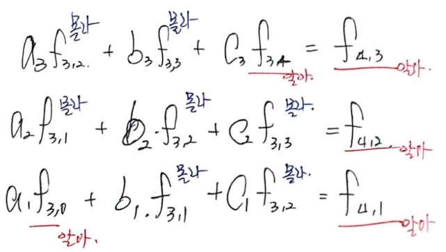
…this kind of shape??????

You see it, right?

Once you write it out like this — 3 unknowns, 3 equations!!!

Ahhh — same number of unknowns as equations, so we can pin down all 3 unknowns, snap snap snap, uniquely.

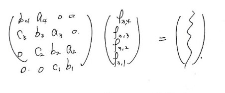
Now I’ll take those 3 stacked equations and rearrange them so that unknowns sit on the left, knowns sit on the right, and write the whole thing as a matrix.

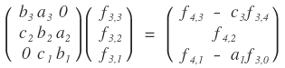
Yo~~~ nice~~~

The vector we don’t know,

just kick that left-hand matrix over to the right as an inverse,

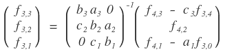
and bam — we’ve got it. heh

Now, one thing that might have you a little suspicious!!!

You might be thinking “OK but this 3×3 matrix only shows up because of this specific tiny example, right?”

Well — let’s see.

If you’ve got 4 unknowns stacked in a column, then in matrix form:

it’d be a 4×4 matrix!!!

100 unknowns? Yeah, you guessed it — 100×100. lol heh heh heh heh heh

OK so in general, you get an $n \times n$ matrix, and to actually solve the matrix equation you need to be able to invert an $n \times n$ matrix…

(annoyed face) (annoyed face)…

So Implicit FDM means we need inverse matrices, which means we need to actually study inverse matrices….

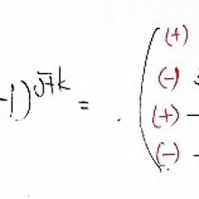
But if you’ve done linear algebra, you already know the move — find the adjoint, multiply by 1 over the determinant, done!!!!

(http://gdpresent.blog.me/220605504163)

Linear Algebra I Studied #15. Adjoint Matrix

Up until now we did determinants for general matrices. Now we look at special matrices. The weird ones…

blog.naver.com

But now I’m sitting here wondering — how on earth do you express that whole adjoint-and-determinant business in code….

Turns out, when a computer inverts a matrix, it doesn’t do it the way you’d do it by hand!!! lol

It’s called LU decomposition!!!!

If I tried to cram LU decomposition in here too, the scroll pressure would be absolutely insane, right??????????????????????

So — next post.

---

Originally written in Korean on my Naver blog (2016-12). Translated to English for gdpark.blog.