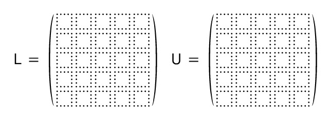
LU Decomposition
Starting from middle-school bike problems and building up to Gaussian elimination, we crack open LU decomposition — because computing A⁻¹ is just painful.
So while we were poking at the Black-Scholes PDE with numerical methods, this thing kept showing up:
$$Ax = b \quad (A: \text{matrix}, \; x \;\&\; b: \text{vectors})$$We want $x$. Easy — just find $A^{-1}$, right?
Yeah, no. Computing $A^{-1}$ is painful, and coding it up is even more painful. So apparently, to make life… slightly less miserable, we learn LU decomposition.
To get LU decomposition, I’m gonna start from Gaussian elimination.
Gaussian elimination, middle-school style
Let me explain the idea at a middle-school level.
You’ve all definitely solved a problem like this in elementary school:
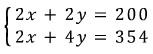
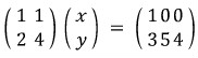
There are 2-wheeled bikes and 4-wheeled bikes, 100 of them total. But for some reason, somebody crouched down and counted only the wheels — and look, it’s already weird that they got an accurate wheel count, but apparently the wheels added up to 354.
How many 2-wheeled bikes? How many 4-wheeled bikes?
(You could’ve just counted the bikes, my dude lol lol lol lol)
Anyway.
When we were kids, we’d start by guessing 50/50, then think “hmm, more 4-wheelers? fewer 4-wheelers?”, and inch our way to the answer.
But the terrifying Korean 8th grader fears nothing. They just slap equations down.
Like this:

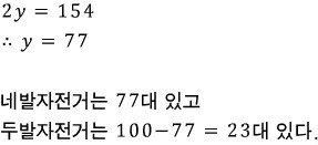
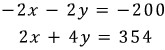
Set up the equations. Then — call it elimination, call it substitution, whatever — they rearrange those two equations into this:
And then this:
And then they just barrel through to the next step like an automated machine:
Now this 8th grader grows up. Goes to college. Takes linear algebra (the required class in basically every STEM major).
And now they’d solve it like this. (Of course nobody actually solves it this way lol lol lol lol)
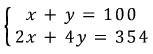
Rewritten as:
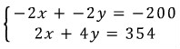
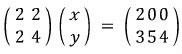
Multiply the top row by 2:
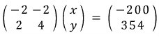
Multiply the top row by $(-1)$:
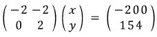
Replace row 2 with (row 2 + that top row):
↓
And replace the top row with (top row + row 2):
↓
Multiply both rows by $1/2$ (and for row 1, also multiply by $-1$):
──── tangent warning ────
If you’re seeing this for the first time, you might be staring at the red arrows above going “…wait, why is that allowed?”
Because I didn’t get it the first time either, heh.
The reason it’s allowed comes down to properties of equality.
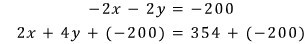
If you have $A = B$, you can add or subtract the same thing $C$ to both sides. Cool.
So in this equation:
think of it like this:
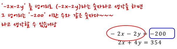
Now let’s clearly add the same number to both sides of the bottom equality. We’ll add $-200$ to both the left side and the right side:
But that $-200$ on the bottom equation? Let’s rewrite it as a different number in disguise:
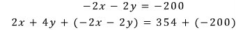
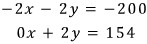
Boom — that’s exactly what those red arrows are doing. You can add or subtract $k$ times one row from another. lol
──── tangent over ────
The compressed version of why all this is allowed: because it’s an equality. That’s it.
But OK, let me say it the fancier way.

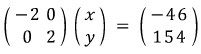
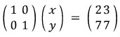
The matrix above ended up looking like this:

But — what if instead it had been (just let this wash over you):
this kind of matrix??????
Through the same “elimination” we just did, it would’ve had to become:
So let me describe what “the form we’re trying to reach” looks like:
And of course this shape, just like above, is reached using only the properties of equality.
For more detail, see http://gdpresent.blog.me/220601043159 .
Systems of equations, Gaussian elimination [ Linear Algebra I Studied #9 ] You all know matrices are systems of equations, right?!?!? Let’s climb up step by step starting from middle-school systems of equations… gdpresent.blog.me
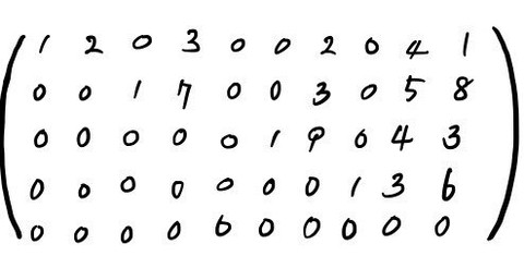
That kind of matrix — with those characteristics — is actually called RREF (Row Reduced Echelon Form). And to turn a matrix into RREF using only properties of equality, you get exactly three moves:
- Multiply a row by a scalar constant.
- Swap two rows (or scale and swap).
- Add a scalar multiple of one row to another row.
That’s it. Those are the only moves. (These three are called the transformation rules.)
Yes yes yes yes yes yes yes — using only these to grind a matrix into RREF is what we call Gaussian elimination.
Don’t lose the thread, by the way: we started from Gaussian elimination in order to learn LU decomposition.
EROMs — the matrices that do the elimination for you
Wow!!!!!!!!
But!!!!!!!!! Here’s the thing.
Those transformation rules I just listed —
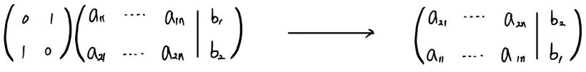
Swapping two rows:
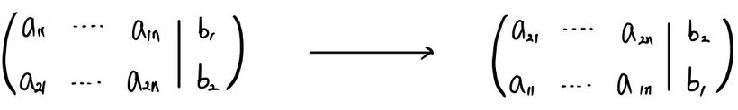
Doesn’t matter, right?? Even doing it like this????
Now check this out — that swap can also be expressed as multiplying by the matrix $\begin{pmatrix} 0 & 1 \\ 1 & 0 \end{pmatrix}$:
Picking one row of a matrix and scaling it:
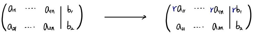
Fine to do without breaking the system, right?
But that scaling is also the same as multiplying by the matrix $\begin{pmatrix} r & 0 \\ 0 & 1 \end{pmatrix}$:
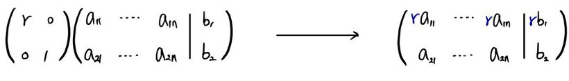
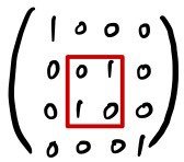
Finally, adding a scalar multiple of one row to another:
Doing this doesn’t break the system either, right?!?!?
But the move is also equivalent to multiplying by $\begin{pmatrix} 1 & 0 \\ r & 1 \end{pmatrix}$:
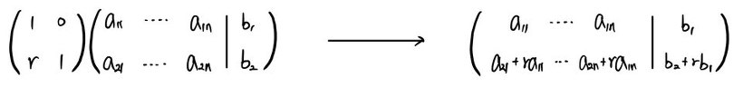
These transformation rules — for a big matrix — are really “pick two rows out of many and do that thing.” That’s why I drew them above as $n \times 2$-ish matrices with two rows.
The point I’m making here is not “eyeball it and figure it out.” The point is:
The act of left-multiplying by a certain matrix is itself the act of applying a transformation rule.
That’s what I want to land.
cf. You might be thinking “OK but does this work for big matrices?” Yeah. Quick 4×4 example so you see it:
To swap row 2 and row 3 in a 4×4:
— same as multiplying by this matrix.
To multiply row 3 by $r$:
— same as multiplying by this matrix.
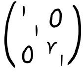
To add $r \times$ row 1 to row 4:
— same as multiplying by this matrix. So yeah, scales fine for any number of rows.
This special matrix — the one that “executes” an elementary row operation when you left-multiply — is called an Elementary Row Operation Matrix (EROM).

From RREF to upper-triangular to LU
So.
If you keeeeeeep multiplying EROMs onto some wild messy not-pretty-at-all matrix (= keep applying transformation rules), it eventually becomes a clean RREF matrix.
But!!!!!!!!! What if RREF is a square $n \times n$ matrix???????
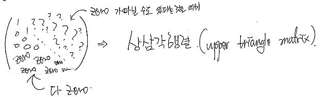
Then can we not call this an upper triangular matrix?!?!

Take a matrix $A$ in some equation, and say it becomes RREF after $k$ transformation rules. That is — say it becomes upper triangular after $k$ rules.
So:

multiplying these EROMs a finite number of times,
— like this — turns $A$ (assuming it’s $n \times n$) into an upper triangular thing. We just confirmed that.
So:

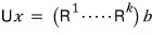
let’s lump that whole stack together —

— like this:
Now — each of those individual $R$’s is, no matter what, an invertible matrix. (Why each one is unconditionally invertible — explaining that would take forever T_T T_T T_T. I’ll outsource to linear algebra… probably you’d want to start from my “Linear Algebra I Studied #8” onward. But to follow #8 you’d want the stuff before #8 too, which is why I’m hesitating to drop a link… so I won’t… heh heh.)
Anyway, so:
what this means is — this is possible.
Yay. OK now —
since this thing becomes a lower triangular matrix,

since this is the conclusion,

it looks like all I have left to explain is why this thing becomes a lower triangular matrix.
First — looking back at the EROMs we just had, every single one of them except the row-swapping EROM was already a lower triangular matrix. → Scroll back up and check!! heh heh
Then two more facts:
The inverse of a row swap is the same row swap. (You swap, you swap again, you’re back.)
The inverse of a lower triangular matrix is also lower triangular.
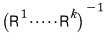
OK so here’s how it really has to be phrased.

In this — instead of applying

in their original order, let’s apply $P$ first (the row swaps).

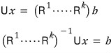
Ah but — in the equation where $P$ has already been fully absorbed,

if we say it was this equation, then now $A$ can, no matter what, be decomposed as $LU$!!!
Yayyyy~~~ $A$ → decomposable into $LU$!!!!
Why we wanted this in the first place
Quick reminder of why we’re doing LU decomposition in the first place.

In a matrix equation, using the inverse:

— this is hell to code.
So instead, since our actual goal is just to find vector $x$:
$$Ax = b$$if we change the equation into the form:
we can find $x$ without ever coding an inverse matrix.

Now the actually hardcore part
OK NOW it gets really hardcore lol lol lol lol lol lol lol
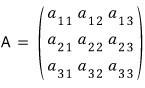
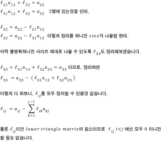
What I mean is: given a matrix $A$, we need to write code that computes the elements of $L$ and $U$ in the LU decomposition.
First —
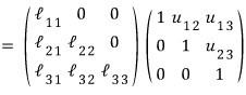
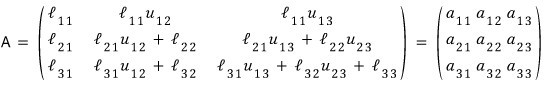
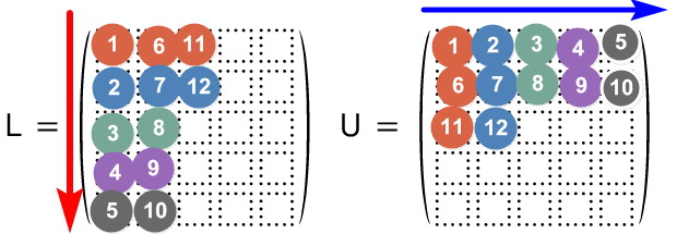
we saw this matrix being LU-decomposed like this:
(Because if you do Gaussian elimination, the leading 1 lands like that in the $U$ matrix?? That is — since I’m assuming the diagonal of $U$ is 1, it’d be more accurate to call this the Crout method.)
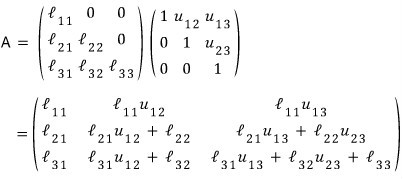
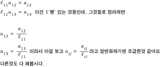
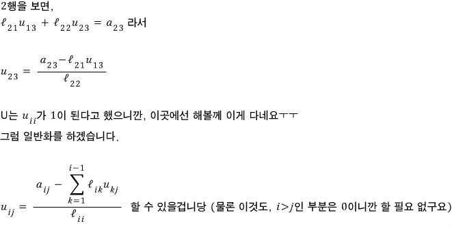
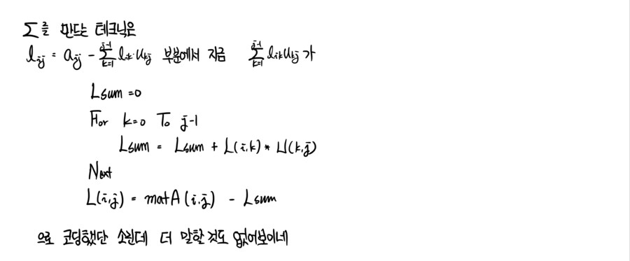
Let’s look at how to code $L$.
What this is saying right now is —

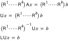
— so we can express $l_{ij}$ in terms of $u_{ij}$ and $a_{ij}$!!!
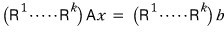
So if you brute-force Gaussian elimination on $Ax = b$, it becomes $Ux = (RR \dots R)b$, and at that point we already know both $u$ and $a$, right?
Since we don’t know exactly what $(RRR \dots R)$ looks like, and finding the lower triangular inverse of it is a pain right now — what this means is, we can just slam $L$ in using only $u_{ij}$ and $a_{ij}$.
Ah but, before coding — that would mean we’d have to do Gaussian elimination on $A$ by hand first and then code, which is also kinda not right.
So from here on, I’m gonna show you what I’ll call the swoosh-swoosh-swoosh calculation method.
Instead of finding everything in one big BANG —
one swoosh from $L$, one swoosh from $U$, then one more swoosh from $L$, one more swoosh from $U$ —
if we go sequentially like that, we can take matrix $A$ and rrrrrrrrrroll right through it, defining every element of $L$ and $U$.
Might be hard to grok at first, but stare at it once and it’ll click lol.
OK let’s go. I’ll explain it with a 3×3 like above, then generalize to $n \times n$.

Looking at this equation first —

— the relationships fall right out.
Pulling them all together:
— let’s call it this.
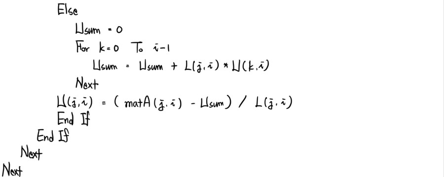
So now what’s left is the $(2,2)$, $(3,2)$, $(3,3)$ entries.
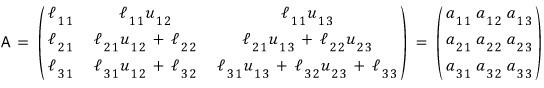
I organized things by $L$; let’s organize by $U$ too.
Looking at the figure again:

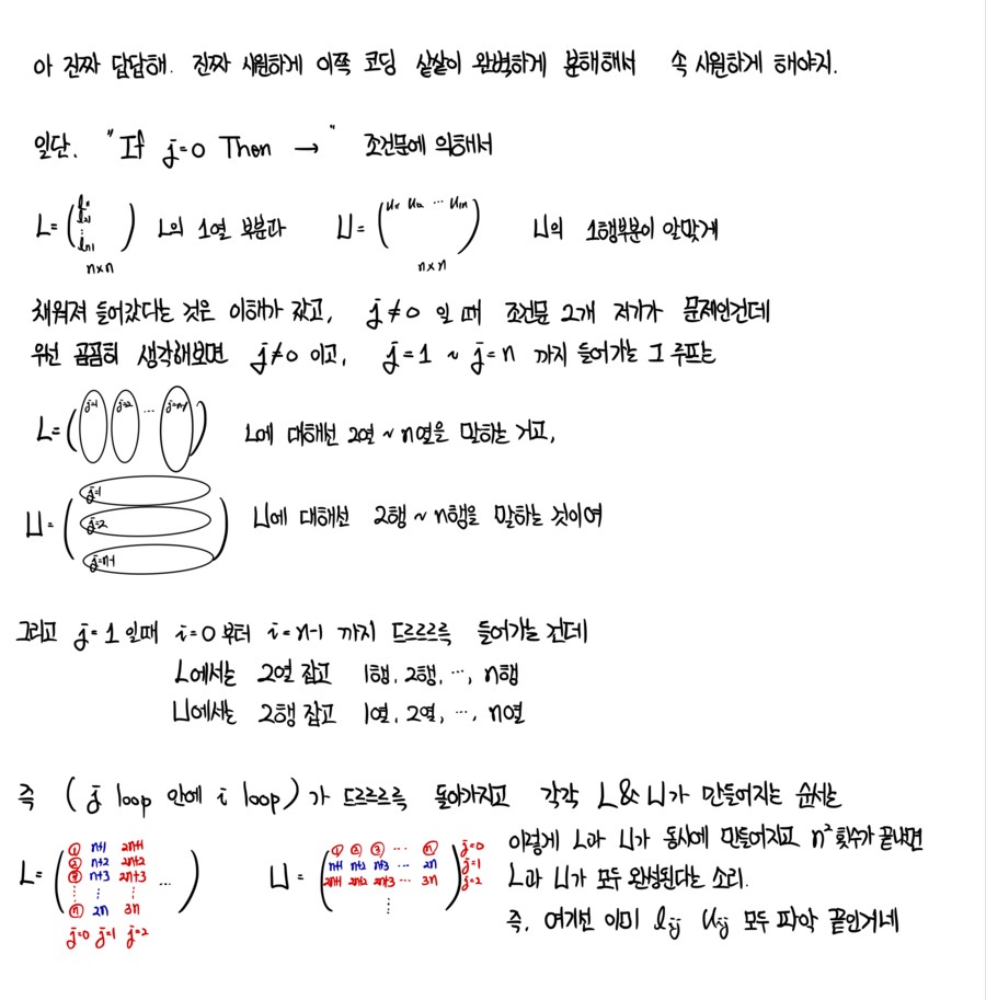
As you can see, $l$ and $u$ are tangled into each other. So when coding, you can’t really do “BANG! finish all of $L$, then BANG! finish all of $U$” — there’s a hard limit to that approach.
The whole point of the swoosh-swoosh-swoosh sequential thing is this:
We already know we can rewrite as $LUx = b$.
And while $L$ and $U$ aren’t precisely known yet,
— this much, we do know.
So then how do we fill the rest in;;;;
When you fill in those blanks — don’t fill in all of $L$~~~ and then fill in all of $U$~~~ — don’t do that.
One from $L$, one from $U$. One from $L$, one from $U$.
Find them in that direction. By rrrrrrrrrolling through it that way, you fill in all of $L$ and $U$.

As the equation shows:
- Column 1 of $L$ can be found from $A$ alone.
- Row 1 of $U$ can be found entirely from the $(1,1)$ element of $L$ and $A$.
- Column 2 of $L$ needs row 1 of $U$. But row 1 of $U$ was already conquered, so → use it.
- Same for row 2 of $U$ — the materials for it were just prepped a step ago. heh heh.
ahaha ahaha ahaha ahaha ahaha lol lol lol lol lol lol lol lol lol
So now we get that you can code your way from $Ax = b$ all the way to $LUx = b$.
Alright — what’s left is heading toward the actual solution vector $x$. Let’s cover that and then look at how the real coding goes! heh heh.
Forward sub, then back sub
I mentioned this briefly above.
──── copy-paste warning ────
Quick reminder of why we’re doing LU decomposition in the first place.
In a matrix equation, using the inverse:
— this is hell to code.
So instead:
Since our goal is to find vector $x$ anyway, if we change the equation to:
we can find $x$ without ever coding an inverse.
──── copy-paste over ────


Mentioned briefly above.
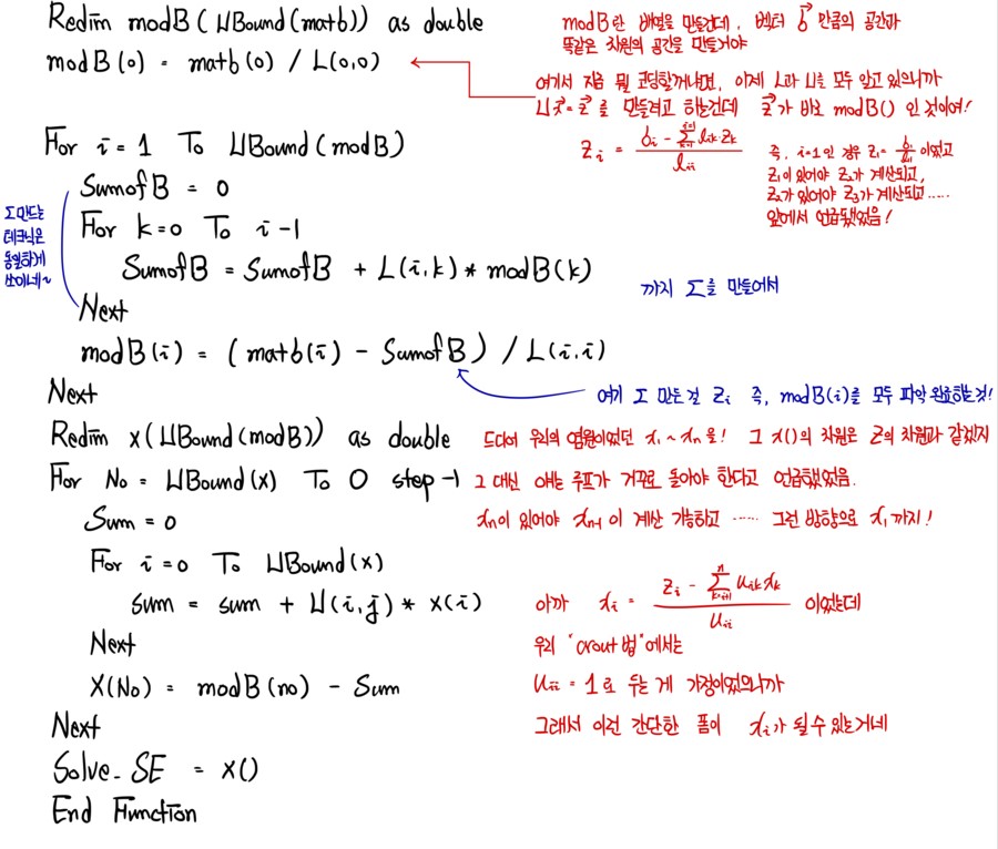
Now that we’ve finished coding $LU$, using the logic above, let’s head toward solution vector $x$.
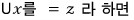
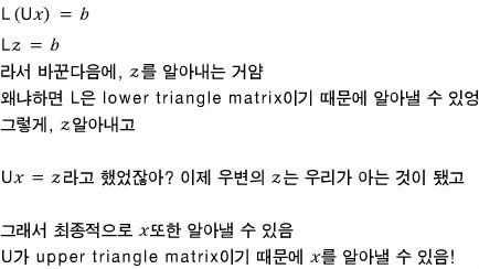
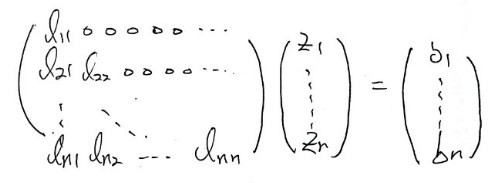
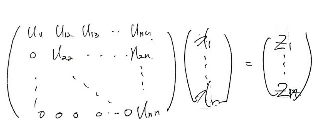
So first let’s set $Ux = z$!!! That makes the equation $Lz = b$, right?!?!
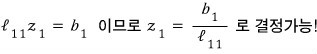
We see it in this form. And since we now know both $L$ and $U$ —
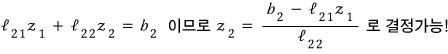
Looking at row 2:
Oh nice — for row 2, since we just found $z_1$, we can find $z_2$ too~~~
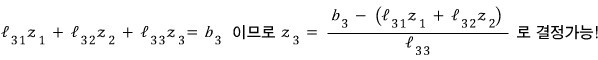
I’ll do row 3 and then generalize.
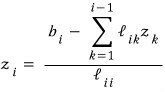
Now generalizing to $z_i$:
That’s the generalization!!! From $z_1$ all the way to $z_n$, sequentially, all found!!!~~~
And now let’s head to $Ux = z$.
We can see it looks like this!
For this one, unlike before, because it’s an upper triangular matrix — that is, because the bottom row has the most zeros — we’ll find things from the bottom up, one at a time. (We currently have all of $z_1$ through $z_n$.)

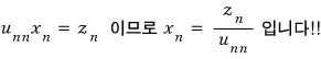
Ooh, $x_n$ pops out!!!
Let’s try the row above:

Ahh — since we have $x_n$, we can find $x_{n-1}$ too!!!
But right now I can’t say it in concrete numbers — I have to keep saying $n$-this and $n$-that. It’s a headache. And generalizing right at this exact step is a bit much, so let me just do one more and then generalize, OK lol lol hoo hoo hoo hoo (T_T T_T T_T T_T).
Next is row $n-2$:
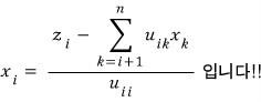
This is so painfully annoying lol hoo… let’s just generalize. Generalize!
Whoa — the principle is finally done?????
The actual code
Now it’s time to code. But honestly… could I have come up with this code myself? (T_T T_T)
I think this is gonna end up being more of a “make sense of code that’s already given to you” kind of session!!
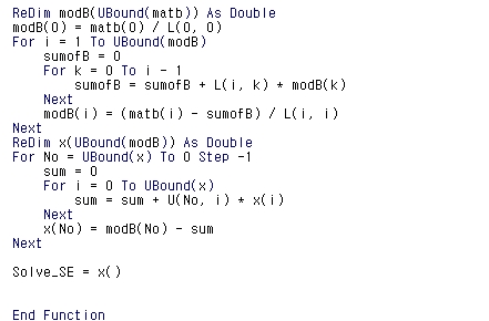
This is a function that, if you just toss in $A$ and $b$ from $Ax = b$, spits out — here’s your solution $x$~~~!
Here it is!
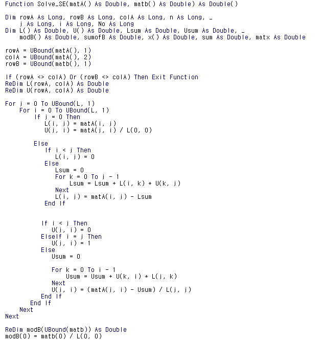
Function Solve_SE(matA() As Double, matb() As Double) As Double()
Dim rowA As Long, rowB As Long, colA As Long, n As Long, _
j As Long, i As Long, No As Long
Dim L() As Double, U() As Double, Lsum As Double, Usum As Double, _
modB() As Double, sumofB As Double, x() As Double, sum As Double, matx As Double
rowA = UBound(matA(), 1)
colA = UBound(matA(), 2)
rowB = UBound(matb(), 1)
If (rowA <> colA) Or (rowB <> colA) Then Exit Function
ReDim L(rowA, colA) As Double
ReDim U(rowA, colA) As Double
For j = 0 To UBound(L, 1)
For i = 0 To UBound(L, 1)
If j = 0 Then
L(i, j) = matA(i, j)
U(j, i) = matA(j, i) / L(0, 0)
Else
If i < j Then
L(i, j) = 0
Else
Lsum = 0
For k = 0 To j - 1
Lsum = Lsum + L(i, k) * U(k, j)
Next
L(i, j) = matA(i, j) - Lsum
End If
If i < j Then
U(j, i) = 0
ElseIf i = j Then
U(j, i) = 1
Else
Usum = 0
For k = 0 To i - 1
Usum = Usum + U(k, i) * L(j, k)
Next
U(j, i) = (matA(j, i) - Usum) / L(j, j)
End If
End If
Next
Next
ReDim modB(UBound(matb)) As Double
modB(0) = matb(0) / L(0, 0)
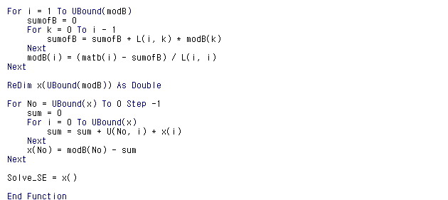
For i = 1 To UBound(modB)
sumofB = 0
For k = 0 To i - 1
sumofB = sumofB + L(i, k) * modB(k)
Next
modB(i) = (matb(i) - sumofB) / L(i, i)
Next
ReDim x(UBound(modB)) As Double
For No = UBound(x) To 0 Step -1
sum = 0
For i = 0 To UBound(x)
sum = sum + U(No, i) * x(i)
Next
x(No) = modB(No) - sum
Next
Solve_SE = x()
End Function
There’s no way to fit this in a single screenshot (T_T T_T T_T T_T), and for it to look like real code it has to be screenshotted, so even when I split it up into screenshots —

I really do think learning to code is something you do solo, going yeong-cha yeong-cha (the grunting-and-pushing sound), but — please just use this as a reference for how I studied the code… ugh.
Continuing:

The VBA results work correctly in Python too.
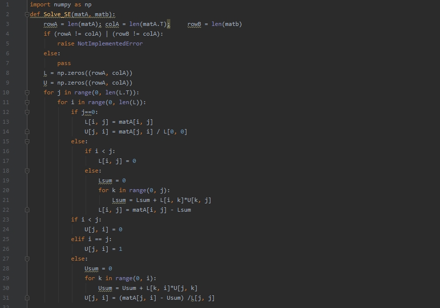

import numpy as np
def Solve_SE(matA, matb):
rowA = len(matA); colA = len(matA.T); rowB = len(matb)
if (rowA != colA) | (rowB != colA):
raise NotImplementedError
else:
pass
L = np.zeros((rowA, colA))
U = np.zeros((rowA, colA))
for j in range(0, len(L.T)):
for i in range(0, len(L)):
if j==0:
L[i, j] = matA[i, j]
U[j, i] = matA[j, i] / L[0, 0]
else:
if i < j:
L[i, j] = 0
else:
Lsum = 0
for k in range(0, j):
Lsum = Lsum + L[i, k]*U[k, j]
L[i, j] = matA[i, j] - Lsum
if i < j:
U[j, i] = 0
elif i == j:
U[j, i] = 1
else:
Usum = 0
for k in range(0, i):
Usum = Usum + L[k, i]*U[j, k]
U[j, i] = (matA[j, i] - Usum) /L[j, j]
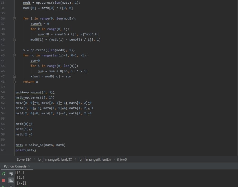
modB = np.zeros((len(matb), 1))
modB[0] = matb[0] / L[0, 0]
for i in range(0, len(modB)):
sumofB = 0
for k in range(0, i):
sumofB = sumofB + L[i, k]*modB[k]
modB[i] = (matb[i] - sumofB) / L[i, i]
x = np.zeros((len(modB), 1))
for no in range(len(x)-1, 0-1, -1):
sum=0
for i in range(0, len(x)):
sum = sum + U[no, i] * x[i]
x[no] = modB[no] - sum
return x
matA=np.zeros((3, 3))
matb=np.zeros((3, 1))
matA[0, 0]=4; matA[0, 1]=-1; matA[0, 2]=0
matA[1, 0]=-1; matA[1, 1]=4; matA[1, 2]=-1
matA[2, 0]=0; matA[2, 1]=-1; matA[2, 2]=4
matb[0]=3
matb[1]=2
matb[2]=3
matx = Solve_SE(matA, matb)
print(matx)
Originally written in Korean on my Naver blog (2016-12). Translated to English for gdpark.blog.