Crank-Nicolson Finite Difference Method (FDM) [Financial Engineering Programming #21]

Now this is the final method we’re covering for FDM.

It’s a concept that sits roughly halfway between the Explicit and Implicit methods we covered earlier, and they say its computation process is the most efficient too,

I’ll mention the reason for that after we’ve gone through all the formulas.

Then let me throw out the Crank-Nicolson FDM method first.

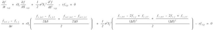
Black-Scholes PDE

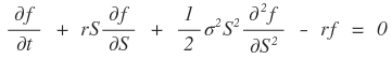
In the partial differential equation above, into the terms corresponding to the derivatives

we plug in approximations like this~

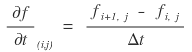
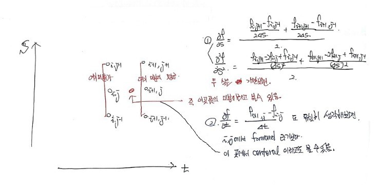
For t we stick with the forward difference,

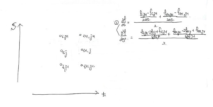
and for the 1st derivative and 2nd derivative with respect to S, we plug them in a slightly weird way~

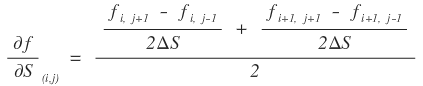
We plug in the average of the central difference centered on j at i and i+1 each~

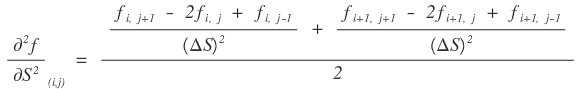
Same here. We plug in the average of the 2nd derivative approximated by the central difference centered on j at i and i+1 each~

Ahahahaha, in order to somehow understand that this kind of approximation is at least a bit “reasonable”, here’s what I thought.

Well, on some arbitrary grid

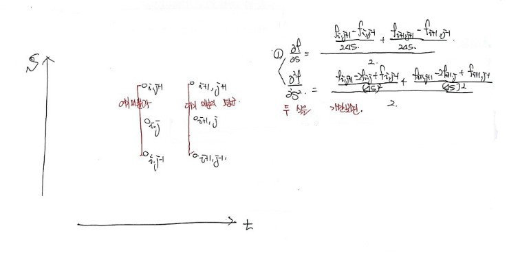
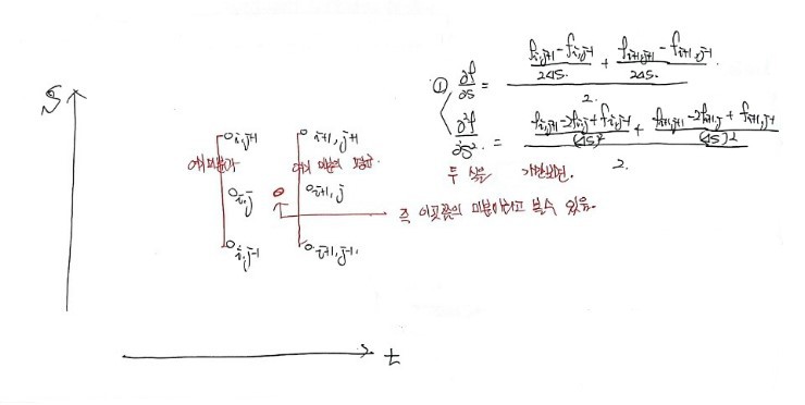
When I thought about it like this, what makes this the most accurate is —

couldn’t this be the method that minimizes the positional error in approximation the most compared to the previous methods —

that’s the kind of thought I had~

OK, so now, let’s plug it nicely into the Black-Scholes PDE as we examined above

and tidy up the equation~

Breaking the above equation into tiny little pieces

and dragging the formula along in as much detail as possible,

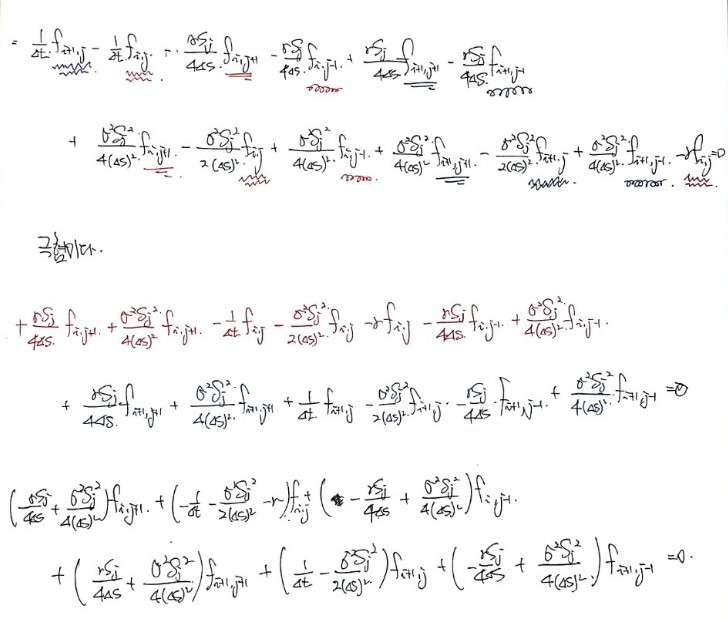
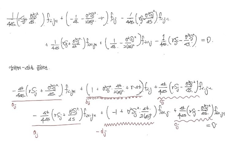
We can bring it down to here and put a period~

It’s more like I did a bit of arithmetic than math, hmm…

Now the way it’s computed is the same as Implicit FDM~

Like with Implicit, let’s say we made the grid 5 intervals each~

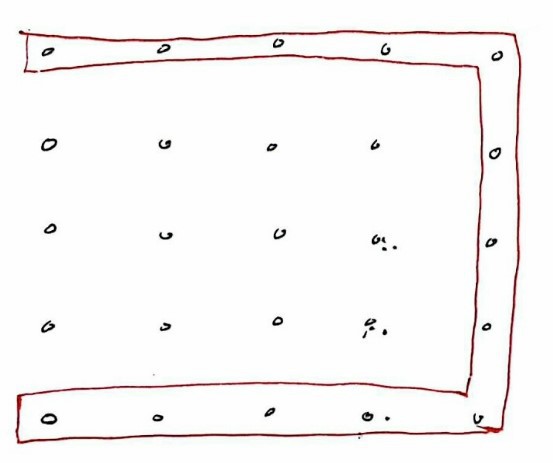
Since we sliced it into 5 pieces,

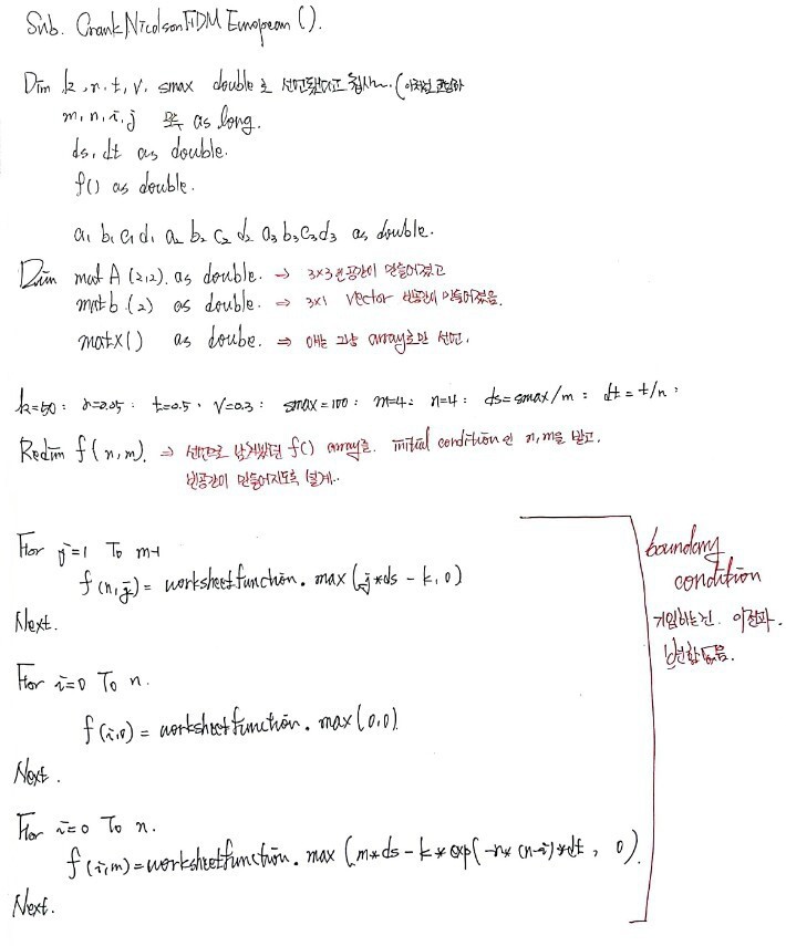
our boundary conditions would now look like this!!!!

In our Black-Scholes approximation,

if we plug in i=3, j=2, we get an equation in those 3 unknowns~

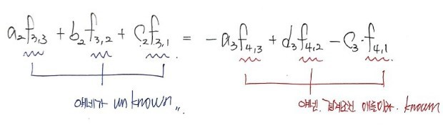
OKOKOKOKOKKOK

But, with just this one equation,

we have 1 equation and 3 unknowns,

so it’s not enough to figure out each-each-each of the 3 unknowns individually.

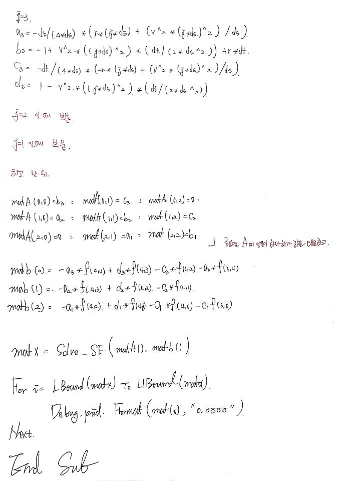
Let me also write the equations for j=1 and j=3,

and then write the 3 equations one after another~

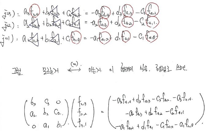
kkkkkkkkkkkkkkkkkkkkkkk

The look of it is for-real revolting kkkkkkkkkkkkkk

It just looks freakin’ complicated;;;

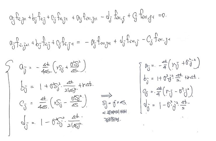
Then now, if we just define a_1,2,3 b_1,2,3, c_1,2,3 & boundary condition

and plug it into our trusty cavalry Solve_SE() function procedure to compute it,

f_3,3 / f_3,2 / f_3,1 will come out, right?!?!?

Right now!!!! Let’s study how this exact situation gets coded~

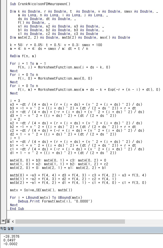
It’s this!!!!!!!

This is how I studied it!!!!

Python version!

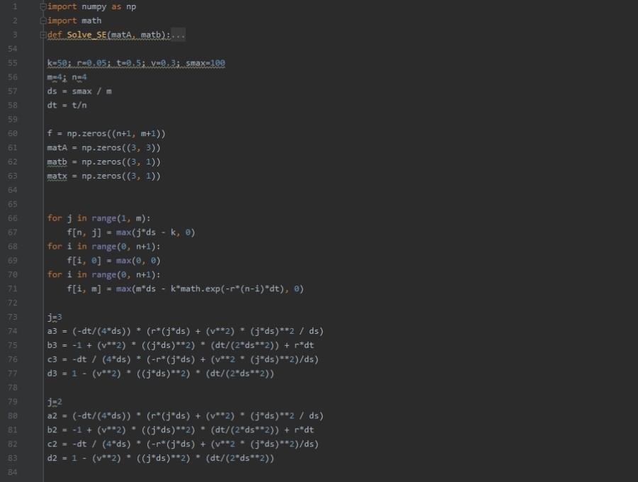
import numpy as np
import math
def Solve_SE(matA, matb):
    rowA = len(matA)
    colA = len(matA.T)
    rowB = len(matb)
if (rowA != colA) | (rowB != colA):
raise NotImplementedError
else:
pass
    L = np.zeros((rowA, colA))
    U = np.zeros((rowA, colA))
for j in range(0, len(L.T)):
for i in range(0, len(L)):
if j==0:
                L[i, j] = matA[i, j]
                U[j, i] = matA[j, i] / L[0, 0]
else:
if i < j:
                    L[i, j] = 0
else:
                    Lsum = 0
for k in range(0, j):
                        Lsum = Lsum + L[i, k]*U[k, j]
                    L[i, j] = matA[i, j] - Lsum
if i < j:
                U[j, i] = 0
elif i == j:
                U[j, i] = 1
else:
                Usum = 0
for k in range(0, i):
                    Usum = Usum + L[k, i]*U[j, k]
                U[j, i] = (matA[j, i] - Usum) /L[j, j]
    modB = np.zeros((3, len(matb.T)))
    modB[0] = matb[0] / L[0, 0]
for i in range(0, len(modB)):
        sumofB = 0
for k in range(0, i):
            sumofB = sumofB + L[i, k]*modB[k]
        modB[i] = (matb[i] - sumofB) / L[i, i]
    x = np.zeros((3, len(modB.T)))
for no in range(len(x)-1, 0-1, -1):
        sum=0
for i in range(0, len(x)):
            sum = sum + U[no, i] * x[i]
        x[no] = modB[no] - sum
return x
k=50; r=0.05; t=0.5; v=0.3; smax=100
m=4; n=4
ds = smax / m
dt = t/n
f = np.zeros((n+1, m+1))
matA = np.zeros((3, 3))
matb = np.zeros((3, 1))
matx = np.zeros((3, 1))
for j in range(1, m):
    f[n, j] = max(j*ds - k, 0)
for i in range(0, n+1):
    f[i, 0] = max(0, 0)
for i in range(0, n+1):
    f[i, m] = max(m*ds - k*math.exp(-r*(n-i)*dt), 0)
j=3
a3 = (-dt/(4*ds)) * (r*(j*ds) + (v**2) * (j*ds)**2 / ds)
b3 = -1 + (v**2) * ((j*ds)**2) * (dt/(2*ds**2)) + r*dt
c3 = -dt / (4*ds) * (-r*(j*ds) + (v**2 * (j*ds)**2)/ds)
d3 = 1 - (v**2) * ((j*ds)**2) * (dt/(2*ds**2))
j=2
a2 = (-dt/(4*ds)) * (r*(j*ds) + (v**2) * (j*ds)**2 / ds)
b2 = -1 + (v**2) * ((j*ds)**2) * (dt/(2*ds**2)) + r*dt
c2 = -dt / (4*ds) * (-r*(j*ds) + (v**2 * (j*ds)**2)/ds)
d2 = 1 - (v**2) * ((j*ds)**2) * (dt/(2*ds**2))
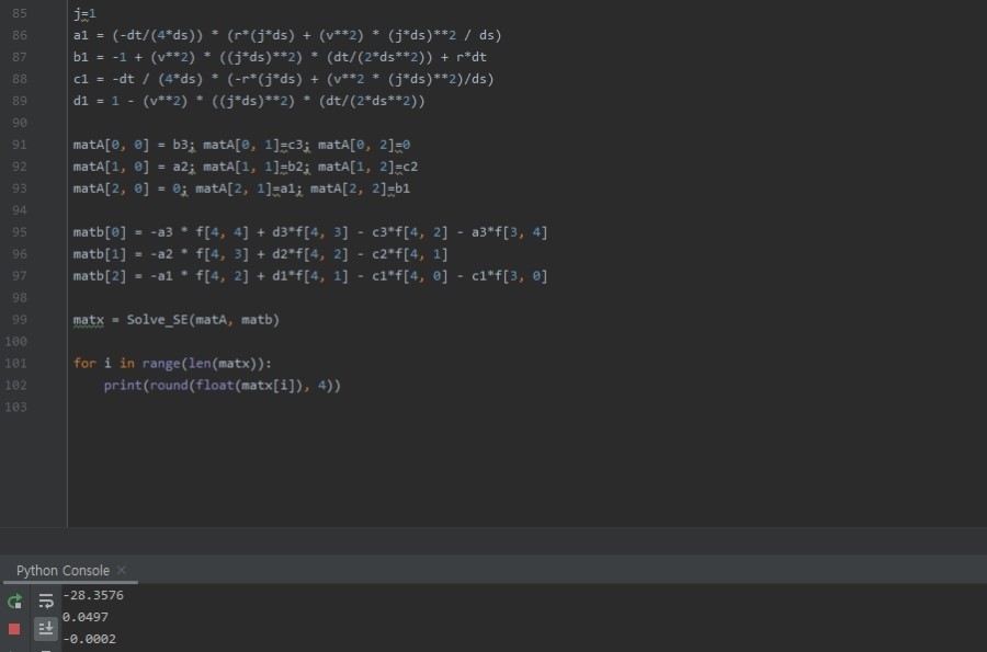
j=1
a1 = (-dt/(4*ds)) * (r*(j*ds) + (v**2) * (j*ds)**2 / ds)
b1 = -1 + (v**2) * ((j*ds)**2) * (dt/(2*ds**2)) + r*dt
c1 = -dt / (4*ds) * (-r*(j*ds) + (v**2 * (j*ds)**2)/ds)
d1 = 1 - (v**2) * ((j*ds)**2) * (dt/(2*ds**2))
matA[0, 0] = b3; matA[0, 1]=c3; matA[0, 2]=0
matA[1, 0] = a2; matA[1, 1]=b2; matA[1, 2]=c2
matA[2, 0] = 0; matA[2, 1]=a1; matA[2, 2]=b1
matb[0] = -a3 * f[4, 4] + d3*f[4, 3] - c3*f[4, 2] - a3*f[3, 4]
matb[1] = -a2 * f[4, 3] + d2*f[4, 2] - c2*f[4, 1]
matb[2] = -a1 * f[4, 2] + d1*f[4, 1] - c1*f[4, 0] - c1*f[3, 0]
matx = Solve_SE(matA, matb)
for i in range(len(matx)):
print(round(float(matx[i]), 4))

Originally written in Korean on my Naver blog (2016-12). Translated to English for gdpark.blog.