Cholesky Decomposition & Correlated Random Variables

This time we’re tackling Cholesky Decomposition.

To get there, I have to do a little math first.

The front half is going to be pretty much pure math, and then I’ll push the financial-engineering side to the back — why we use Cholesky in financial engineering, how we use it, that whole thing.

OK so. A real matrix is…

a matrix that comes back as itself when you apply complex conjugation. That’s it.

Like this. A matrix with that property is a real matrix.

(Basically: it just has real entries.)

Now there’s also a kind of matrix that comes back as itself even after you take both the complex conjugate and the transpose:

Doing transpose-and-complex-conjugate together is called taking the dagger (which is why the symbol is, well, a dagger).

If you dagger it and get the same matrix back, that matrix is Hermitian — a complex symmetric matrix.

But honestly — the matrix we’re going to be dealing with from here on is a covariance matrix. And where on Earth would a complex number show up in a variance???

So instead of the full Hermitian definition, I’m going to work one step narrower: the Hermitian-of-real-symmetric case.

If A is real symmetric and

we call it that.

We’re not going deep on all of this though. We’ll just glance at positive definite and move on. Why? Because the matrix we’re about to handle is a covariance matrix, and a covariance matrix has no choice but to be positive definite.

What’s a covariance matrix???????

I’ll cover it in my financial management posts. Haven’t written that one yet, but I’ll get to it in the next few days, and the second it’s up I’ll drop a link here. — done, linked it :)

Minimum Variance Portfolio — Financial Management I Studied #10 Picking up right where the last post left off. No intro. Alright then, diversifying into this and that…

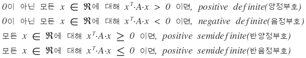
OK let me just throw a couple of theorems about positive definite at you.

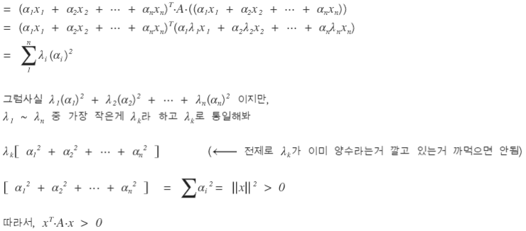
Theorem 1. A is real symmetric. Then the necessary and sufficient condition for A to be positive definite is that all eigenvalues of A are positive.

proof. Suppose A is positive definite, λ is an eigenvalue of A, and x is any eigenvector corresponding to λ. Then

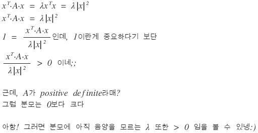
We also need the other direction.

Suppose every eigenvalue of A is positive. Take the set of eigenvalues of A:

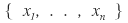
And for any nonzero vector

which is

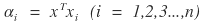
and any vector can be written as a linear combination of

That is,

Then

is

OK — but isn’t requiring a matrix to be Hermitian or real symmetric kind of restrictive? Like, are there even that many of those, what’s the point…???

Nope, not at all. In physics, Hermitian shows up everywhere. Especially in quantum mechanics… god, I hated it… ;_;

A few more properties: if A is Hermitian and positive definite → A is invertible. Also, if A is Hermitian and positive definite, then det(A) > 0. That kind of stuff.

I was going to write all six properties out, but I think I can get to Cholesky decomposition without the rest of them, so I’ll skip and move on. heh. If you’re curious, crack open any linear algebra textbook.

OK, on to Cholesky.

We did LU decomposition before, right? You can basically think of Cholesky as just doing LU decomposition. Except — the assumption on A this time is different. The A we’re going to LU-decompose here is Hermitian (since it’s a covariance matrix) and positive definite.

(From here on this builds on the LU decomposition post, so leaving that link.)

LU decomposition — Financial Engineering Programming I Studied #19 In the process of understanding the Black-Scholes PDE through approximate numerical analysis, Ax = b (A: matrix…

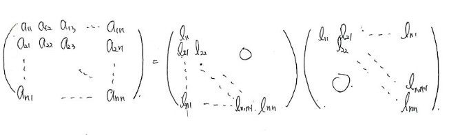
When you decompose this kind of A, it looks like this:

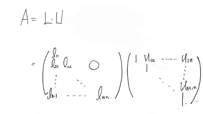
And because A is symmetric, $l_{i,j}$ and $U_{j,i}$ have to be equal. So we can write it like this:

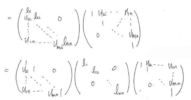
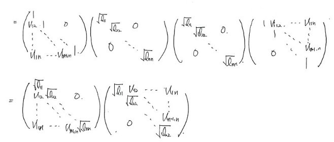
And in the end:

This decomposition is what’s called Cholesky Decomposition.

So why does it matter? First reason: when you want to solve $Ax = b$, even if A is Hermitian and positive definite, using the regular LU decomposition algorithm we used before takes — apparently — about twice as long compared to using an algorithm built on Cholesky. Since we want our code as minimal as possible and faster is better, that alone is enough reason for Cholesky to matter.

But that’s actually not the reason we care about Cholesky here.

Hmm… OK, something I need to lay down first. We’re planning to work with a covariance matrix. It’s painfully obvious that a covariance matrix is symmetric. And as for being positive definite — well… if a covariance matrix weren’t positive definite, that would mean the variance of returns could come out negative…

Variance? Negative??????????

That makes no sense. So a covariance matrix has no choice but to be positive definite.

We’ll write the covariance matrix as Σ, and we’re going to put Σ to work. As established, Σ is Hermitian and positive definite, so Cholesky decomposition is on the table:

And the piece of this we’re actually going to use is L. The lower triangular matrix!!!!

Why are we using L??

To inject correlation into stock price movements.

See, there’s a problem with everything we’ve learned up to this point. Stock price movement is random — yeah, sure — but when you look at two stocks at once, say Hyundai Motor and Kia, both are independently Gaussian-random, so if you just sketch them like this:

— just sloppily independent like that — that probably doesn’t match reality. The two stock prices are individually random, true, but when you look at them together, it’s more accurate to say they’re random in a way that’s correlated with each other…..

So now we want to draw two random variables, and we want them to be random in a somewhat-correlated way. Random variables like that are called correlated random variables (yep, exactly what it sounds like).

Back in the day we learned how to draw random numbers $\varepsilon \sim N(0,1)$. But here, if we just draw two of them and use them as-is:

it’s a little inappropriate. So we transform these two appropriately

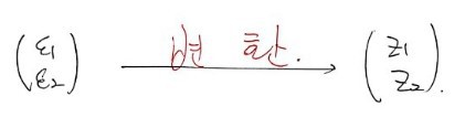
and we want to come out the other side with $z_1, z_2$ — correlated random variables, drawn randomly but with some correlation baked in!!!!

That’s exactly where we use the L matrix from

!!!!!!!

Like this — multiply ε by L, get $z_1, z_2$ out!!!!!

But then why does

actually produce correlated random variables??!!

Honestly — I myself can’t prove this cleanly with math……

BUT!!!!!!!!!!!!!!!!!!!!!!!!! If we draw $z_1, z_2$ a huge number of times, reconstruct $\mathrm{cov}(z_1, z_2)$, build the covariance matrix from those samples, and then show that what comes out is exactly Σ again — wouldn’t that be ironclad?????????????

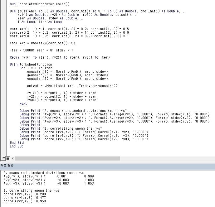
We can verify it with this code!!!!!

We pick one specific covariance matrix:

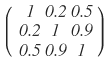
and a function called Cholesky() runs the decomposition on it (how to write that function is coming up right after this), and then using MMult we multiply Gaussian-drawn random numbers $\varepsilon_{1,2,3}$ by the L that came out of Cholesky.

Then $z_{1,2,3}$ — referred to in the code as rv() (I’m guessing for “random variable”) — get drawn many times, equal to the iteration count, and we have the code recompute their means, variances, and the pairwise covariances for (1,2), (1,3), (2,3). And we could confirm that exactly the covariances we put in came back out.

What were we trying to confirm again???? — that we really did take the covariance matrix Σ,

ran Cholesky on it like this, took the resulting L,

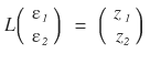
used it like this, and the random variables $Z_{1,2}$ that pop out really are correlated with each other?!?~~~

Result of the check: confirmed. heh.

Alright, moving on. lol lol lol lol lol

OK — now let’s tackle the part we glossed over: the algorithm that actually produces L from the input matrix. Let’s wrap with that.

Say the Cholesky decomposition looks like that.

Start with $a_{11}$. Obvious at a glance:

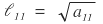
Something like this?!?!?!

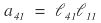
Now look at $a_{21}$. Multiplying row 2 of the front matrix by column 1 of the back matrix gives $a_{21}$,

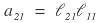
and everything except that one term gets wiped out.

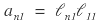
Wait?!?! Come to think of it,

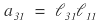
same deal with this one,

and same with this one too, so

we can write it like this.

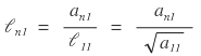
Ah, in that case

we can write it like this!!!!

Column 1 of L: done. On to column 2.

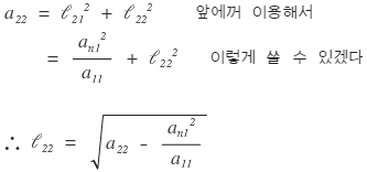
Multiplying row 2 (front) by column 2 (back) all the way through gives $a_{22}$, so

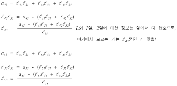
Next we’d normally look at $l_{32}$, but let me peek at $l_{33}$ and $l_{44}$ real quick first.

Ah — now I can see the pattern.

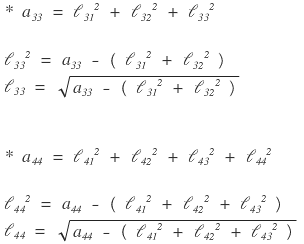
We can write it like this.

And looking at row 3 (front) times column 2 (back),

it looks like we can generalize column 2:

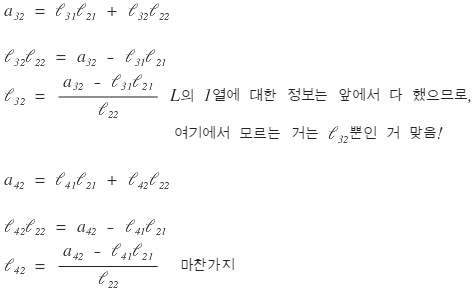
Let’s check column 3 too:

Yep, column 3 generalizes too:

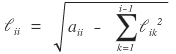
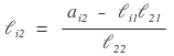
And looking at it all laid out like this, it looks like we can write a single formula for every $(i, j)$ of L!!!!!!!!!!!!!!!!!!!!!!!!

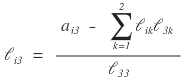
Like this!!!!

Of course, since L is lower triangular, every $(j > i)$ entry is 0. heh.

And — as I noticed while deriving this just now — looks like we have to fill in L sequentially: column 1, then column 2, then column 3….

Alright, since we roughly get the principle, let’s look at the function procedure that spits out L after Cholesky decomposition!!!

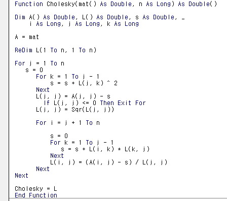
It’s short and clean. Like… honestly, there’s not really anything more to study here.

OK — now we can generate the stock-price movements of two or more stocks. For two-or-more stocks, we calculate their covariance, plug the covariance matrix into the code above, extract L, take the linear combination of L with the Gaussian-drawn $\varepsilon$, get Z out, and then generate stock prices using exactly the same machinery from the Monte Carlo Method post.

Monte Carlo Method — Financial Engineering Programming I Studied #9 It’s that “the more you do it, the closer to the mean it gets” thing. Similar to the Law of Large Numbers…

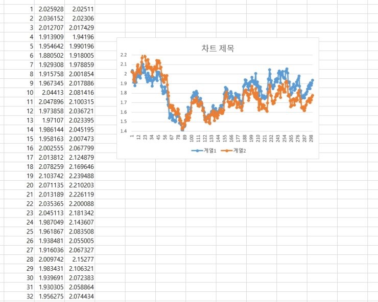
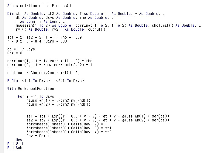
As an example, let’s try it. Plug in a correlation coefficient of 0.9:

Run it:

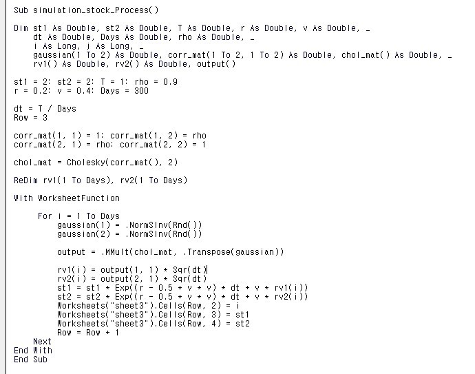
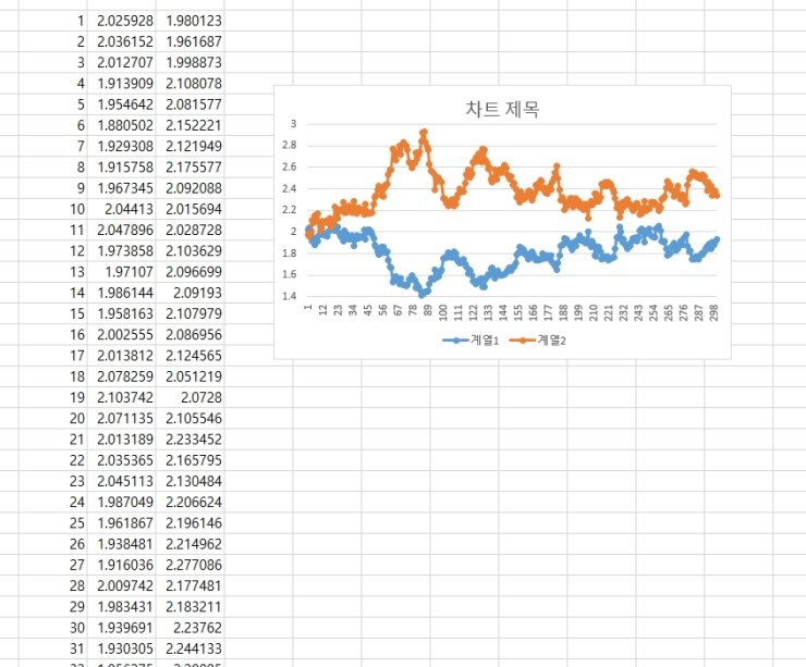
Generated like this. I thought that was kind of cool, so I tried sticking in -0.9. With $\rho = -0.9$, the two stocks should move in nearly opposite directions, right?

I literally only changed the rho slot to = -0.9??????????

Whoa. Magic. Wild. lol lol lol lol lol lol lol lol lol lol lol lol

lol lol lol lol lol lol lol lol lol lol lol lol lol lol lol

I’m pumped lol lol lol lol lol lol lol lol

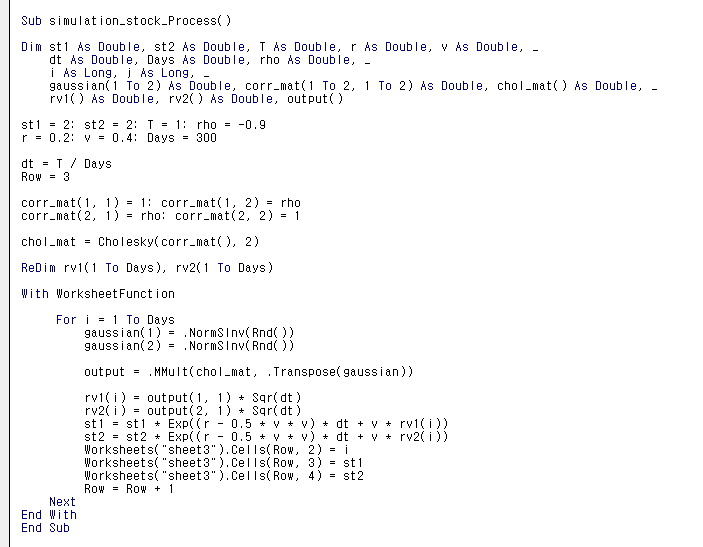
OK and now, instead of generating $z_{1,2}$ to drive the stock prices, I just let the independent random numbers $\varepsilon_{1,2}$ drive them directly.

Here’s the part of the code I touched:

Inside the for-loop, I deleted the rv variable and dropped the Gaussian variable in instead. That way $\varepsilon_{1,2}$ goes in where $z_{1,2}$ used to, right?

Ah, this is fun lol lol lol lol lol lol

Wild lol lol lol lol

Anyway, I’m done now.

Let’s see if I ever study financial engineering again. (-_-)

Originally written in Korean on my Naver blog (2016-12). Translated to English for gdpark.blog.