Systems of Linear Equations and Gaussian Elimination

Everyone knows matrices are basically systems of equations, right?!?!?!!!

So I’m gonna walk through systems of equations step by step, starting all the way back at the middle-school level.

(If a middle schooler actually reads this, they might experience a continuous chain of total mental breakdowns and trip a circuit breaker lol lol lol lol lol lol lol lol

I’m talking from middle-school-GD’s perspective here, but apparently these days there are tons of middle schoolers already doing uni-level stuff???!!!)

OK OK OK OK OK. First off — what even is an equation?!?!

“An equality with unknowns in it!!!” Right. So whenever we run into an equation, our goal is crystal clear:

“Find the unknowns that make the equality hold.”

(For reference — when we run into a differential equation, the goal becomes “find the function that makes the equality hold.”)

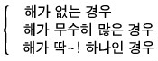
Anyway. When we sit down with an equation and try to find its solution, the outcome falls into one of three buckets.

Quick aside.

The case where there are infinitely many solutions —

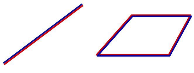
Like on the left: you can have infinitely many because two lines overlap, and you can also have infinitely many because two planes overlap.

Both are “infinitely many” — sure — but even within infinity, there’s gotta be a hierarchy, right? Like, surely the case where two planes overlap and give infinitely many should have more solutions than the case where two lines overlap and give infinitely many, right?!?!?!

Conclusion: they’re the same.

Explaining this here would take forever.

Just accept it and roll with it.

(What it really says is — you can build a one-to-one correspondence between the two solution sets.)

Now, in linear algebra — same as in high school — we’re not messing with degree 2 or degree 3 stuff.

Say there are $m$ first-degree equations.

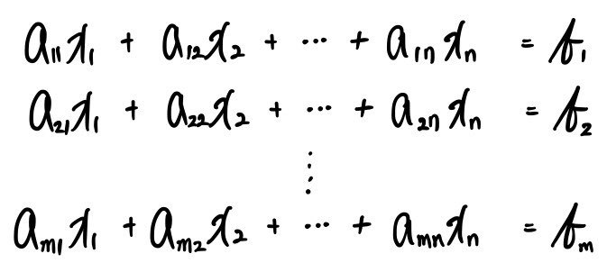
If we rewrite this in the matrix form we’ve been using all along, we get this:

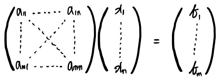
Which we can write as $AX = B$, right?!?!?!?!?

And this matrix $A$, well —

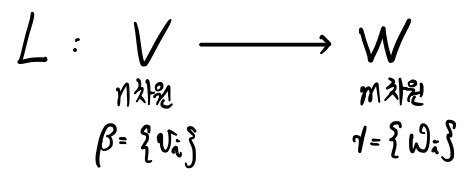
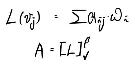
we can call it a matrix representing a linear map $L$, like this,

and as we learned earlier, we can also write it like this:

OK — now I’m gonna split linear systems of equations broadly into two types.

In $AX = B$ above:

the case where $B$ is $0$, and the case where $B$ is not $0$.

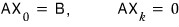
That is — $AX = 0$ vs. $AX = B$.

The former is called a homogeneous equation, and the latter is called a non-homogeneous equation.

(For reference — in a non-homogeneous equation, “non-homogeneous” means $x^1$ (degree 1) and $x^0$ (degree 0) are mixed together, so it’s not homogeneous. That’s why we call it non-homogeneous.)

You gotta understand the homogeneous case before you can solve the non-homogeneous one,

so let’s poke at the homogeneous equation first.

Properties of the homogeneous equation

→ The defining feature of the homogeneous equation: the solution set forms a vector space.

The set of all $X$’s satisfying $AX = 0$, gathered up together, forms a vector space~~~

Let’s see why.

and

Say these are elements of the solution set.

Meaning — each of them satisfies

,

right?!?!?!?!

Oh but —

is also a solution!!!!!

And of course

,

,

and a bunch of other scalar multiples are also solutions.

Hmmm~~~ and for the homogeneous equation, there’s one solution we can spot right away.

Among all the $X$’s that satisfy the equality, the easiest one to pick out is $X = 0$.

Right?! $X = 0$ obviously satisfies it, so yeah — it’s a solution.

But like… what does $X = 0$ even mean as a solution? Nothing. Means nothing at all.

A solution like that is called the trivial solution.

So really, the goal with a homogeneous equation is to find the non-trivial solution!!!!

OK anyway — we wanna find $X$ satisfying $AX = 0$.

But wait?!?!?! This $X$ that satisfies the equality —

that means: when we hit vector $X$ with matrix $A$, it sends it to $0$.

Whoa?!?!?!?!!!

So can we say the solution set is the kernel of $A$?!?!

Well — not quite. The $X$’s belong to the kernel of the linear map $L$ that matrix $A$ represents —

we can say that, right?!?!!!!

I’ll write it like this.

Here’s the punchline.

The solution set can be written as $\ker A$, and $\ker A$ is obviously a subspace, right?!?!?!

That is — we already know the kernel is a vector space.

Which means: the defining feature of the homogeneous equation is that the solution set is a vector space!!!!

Properties of the non-homogeneous equation

OK now let’s look at the non-homogeneous case.

Say there’s an element of the solution set satisfying $AX = B$:

Ahhh~~~ but when we look at matrix $A$, there can be a kernel, right?????

Let’s also say there’s an element of $\ker A$:

That means

right?!!

You can already see where this is going.

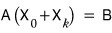
is also in the solution set.

So the solution set is

OK OK OK OK — but —

we assumed there exists a particular solution

right?!?!?!

If no particular solution like that exists, nobody in their right mind would answer “the solution set is $\ker A$.”

That is — if there’s no particular solution, the solution set is just the empty set.

So now we know what the solution set looks like —

but as I wrote at the very top, the number of elements in the solution set can be 0, can be 1, or can be infinitely many, right???

Right now we’ve got a particular solution, a kernel, and the three cases we learned in high school.

This might all sound like total nonsense at the moment,

so let me recycle the words above at high-school-math level.

Then you’ll see what every single one of those words actually means.

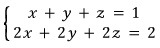
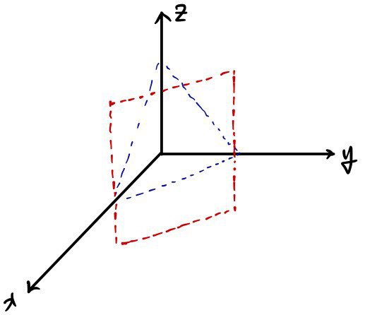
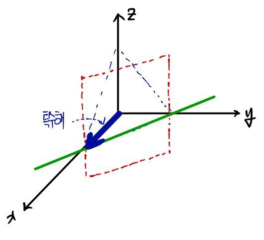
What’s the solution to this system?!?!?!?!!!!!

Yeah — exactly.

It’s a plane.

This kind of plane —

no no — every point lying on this plane is a solution!!!!!!!

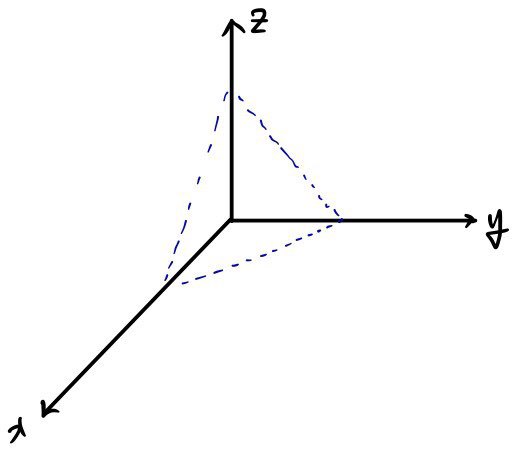
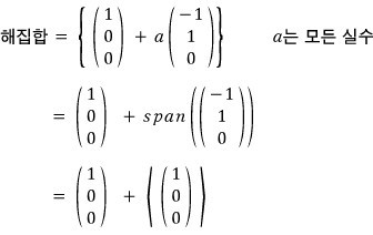
So we can describe the elements of the solution set like this.

Every individual point!

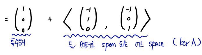
But what the above is really saying is:

This particular solution, plus

a linear combination of the general solutions —

i.e. the solution set can be expressed as a span.

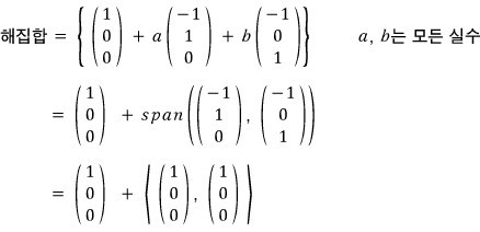
(Note: span is often written with brackets — angle brackets.)

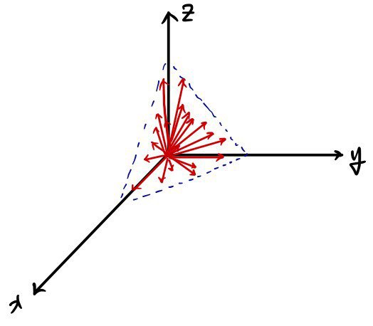
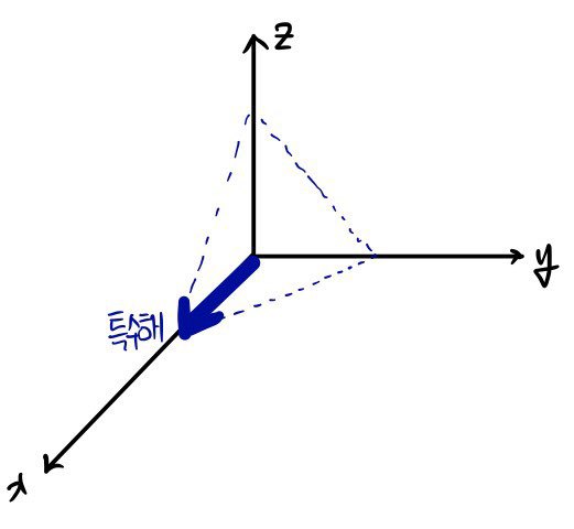
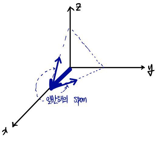
Let’s also look at this system.

Since it’s the line of intersection of these two planes,

this line is the elements of the solution set.

Using this particular solution, plus

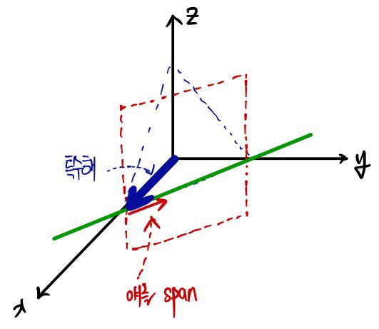
if we span this guy, we can express it!!!

The difference between the solution sets in the two examples —

it’s that the dimension of the vector space called Kernel is different?!?!?!!!!!

Keep that in your back pocket as we move on.

Note) When we hit a homogeneous equation, our job was to find the non-trivial solution — but how do we even know whether one exists?!

“Under a special condition, it has to exist!”

That special condition is

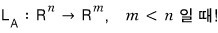
that is — when the matrix is wider than it is tall

= when there are more unknowns than equations!!!

The proof is apparently easy using the dimension theorem.

The dimension theorem says

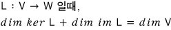
Here, $\dim \mathrm{im}\, L$ is at most $m$, right???? So $\dim \ker L$ —

at smallest, is $n - m$.

But our condition says $m < n$,

so $0 < n - m$, right!

Which says $\dim \ker L > 0$.

And $\ker L$ is the solution set of the homogeneous equation,

so the fact that the solution set has dimension at least 1 means there’s some element other than $0$ —

and that is exactly the non-trivial solution~!

Now I’ll show you the method for actually finding the solution.

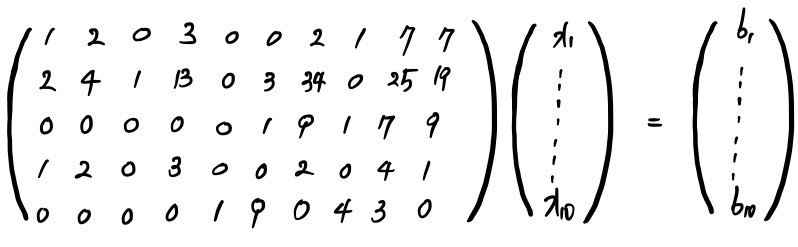
When we’re staring down a matrix this size,

is it just impossible to find the solution because it’s too big?!?!?!!

No no — it’s possible, it’s possible.

It just takes forever!!!!

Like — it is absolutely not something that can’t be found.

OK, here’s the method!!!!

Gaussian Elimination (GE)

That matrix above is, of course,

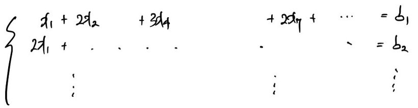
a system of equations like this, written in matrix form.

So now….

To solve that matrix, do we have to convert the whole thing back~~ into equations,

then multiply by constants and add and subtract like we did back in middle school…..

Gaussian elimination is kinda similar (same concept, really) —

but it lets us finish things off more easily, right inside matrix form.

First, let me run Gaussian elimination on an elementary-school-level equation.

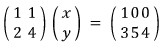
There are 100 bicycles in total — some with two wheels, some with four —

and when we count just the wheels, there are 354.

How many two-wheelers and how many four-wheelers?!

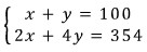
We’d set it up like this, right???

I’m gonna write this step by step as a matrix, and then as the matrix representing the system.

Apparently this matrix form is also written like this:

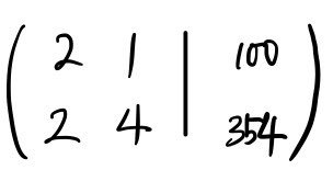
We just rewrote it in a different layout, and the rules of equality still apply,

so we can write it as

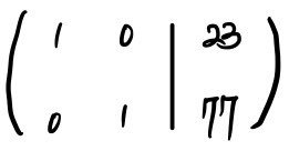
This is Gaussian elimination in action.

It’s literally the same thing, isn’t it…….. T_T T_T T_T

No…. actually there are a few rules, but this example is too simple to really show them off……

Anyway — the principle is exactly the same as elementary school!

So now,

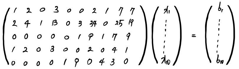
for a giant 5×10 matrix like this, we multiply rows by constants, add and subtract rows

(same idea as the old way of solving equations) and clean it up.

Where exactly?! Until when?! do we have to keep cleaning — that is precisely

the rule of Gaussian elimination,

but talking about that rule right here feels like a bit much.

I think it’ll click better if I cover it afterward,

so I’ll continue with how to actually do Gaussian elimination in the very next post!!!!!!

So for now,

here’s what it looks like once everything is cleaned up all the way:

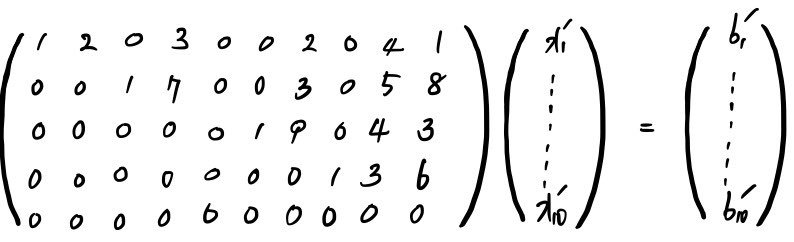
This is the cleaned-up form!!!!!

Eyeballing it — you get the feeling that there’s a lot of 0’s, and roughly if you draw a diagonal, everything below the diagonal is 0… that kind of vibe.

But if you actually write out this matrix as its corresponding system of equations, you can really feel how clean things have gotten.

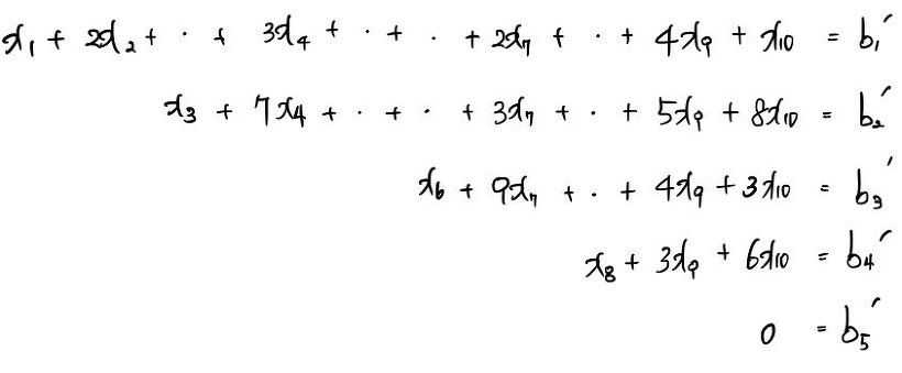
The far-right side got cut off. It’s $0 = b'_{(5)}$.

OK, let me list the characteristics of the matrix above.

① Every single row starts with 0!!!! And the first non-zero element to show up is always 1.

② Rows that are entirely 0’s are stuck at the very bottom, hmm???

③ Now, look at the columns where the first 1’s (the Leading 1’s) live — everything else in those columns is 0?!?!?!

When all three conditions hold, we can call the matrix sufficiently clean.

With a clean matrix like this, we can see the solution at a glance~~~!!

Huh?!?!? So what is the solution then?

Let me give it to you up front.

Move everything that isn’t tied to a ’leading 1’ over to the right-hand side and write it out.

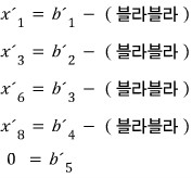
Note) If $b'_{(5)} = 0$ doesn’t hold, the solution set becomes the empty set!!! Watch out, watch out.

The above isn’t just the answer~~~~~~!!! — let me write it out as the full solution set.

The thing about the variables $x'_{(1)}, x'_{(3)}, x'_{(6)}, x'_{(8)}$ tied to the leading 1’s is —

once the values of all the other variables are pinned down, these guys are immediately fixed.

Think about it for a sec. Writing $x'_{(7)} = $ something would be weird.

Because $x'_{(7)}$ shows up in tons of other rows too… that’s what’s going on here.

Those variables don’t affect the other rows.

Those variables are dependent on the others!!!!!! That’s what I’m trying to say!!!!

So those guys are called dependent variables, and the ones up there — $x'_{(2,4,5,7,9,10)}$ — are called independent variables~

Starting at $x'_{(10)}$ and walking upward one by one to grab the elements of the solution set is no effort at all.

These are independent unknowns, so you can plug in whatever values you want. Just stuff values in freely and tweak them so the equation is satisfied.

And this gloriously convenient matrix form is called the Row Reduced Echelon Form —

from here on out, I’ll just call it RREF, taking the first letters of each word above.

Originally written in Korean on my Naver blog (2016-01). Translated to English for gdpark.blog.