Determinants

OK so up to now, think of everything we’ve done as background-building. Now it’s actually time to find the Determinant! Time to learn how to determine the value, exactly!!!

If you keep at it~~~~,

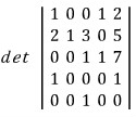
you’ll be able to crack this determinant too. Right now it probably feels like “whoa?!?! no!?!? THAT?!?! HOW!!!”, right? It’s actually super easy, lol. Let’s go!

You haven’t forgotten where the determinant came from, right?!

Yep — it came out of the Alternating Form, one flavor of Multi-linear Forms. That was defined like this:

And from there, the definition of the determinant of an $n \times n$ matrix was that part out front (the Alternating form with $\mathrm{Al}(I_n) = 1$, so each $\mathrm{Al}(e_{i_1} \cdots e_{i_n})$ is just the epsilon symbol $\epsilon_{i_1 \dots i_n}$).

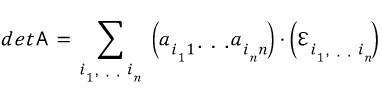
Like that!!! Right?!

Size up step by step

OK then let’s size up step by step, starting with a 2x2!!!!

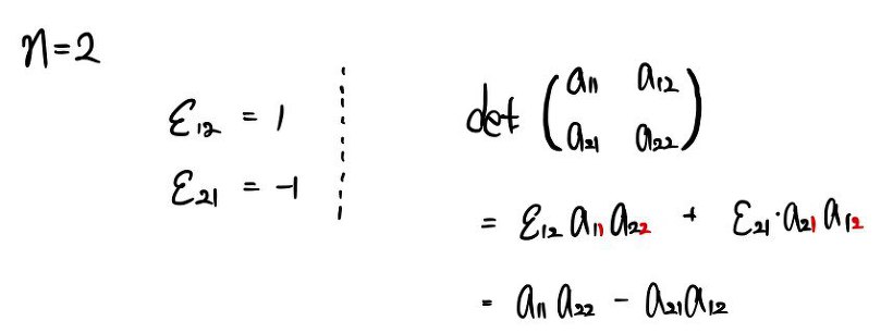
I deliberately used subscripts and red and black colors… to make it easier to follow… (sob)(sob) I’m honestly worried it might be making the breakdown worse. On the left I cleaned up the epsilon symbols, and on the right I ran the calculation using the determinant definition from above.

Let’s do 3x3.

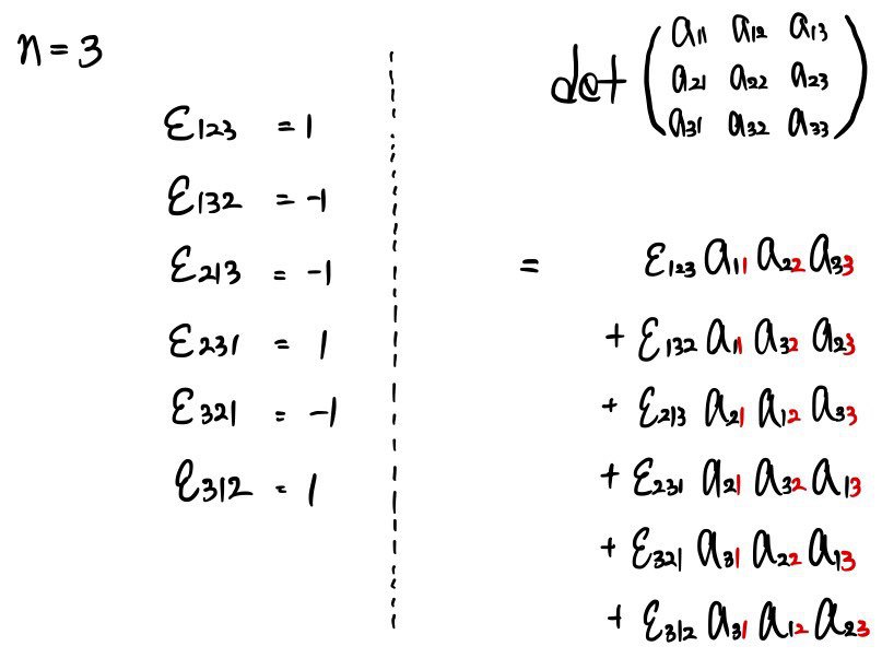
Same principle as above. 3-by-3 shows up a ton — anytime we deal with 3 dimensions, or tensors — so this one’s not bad!!!! We already know it’s calculated like a cross product!!! That’s how Curl gets calculated too, right?

I think we should not forget that this thing we’ve been doing all along without thinking actually originally came out of the Alternating Form.

(I’m a physics student, so when I found this part out I was seriously like lol, what lol, so THIS is what it really was~~~~ and I just collapsed lol lol)

Now, the 4x4

OK now let’s go to 4x4!!!!!!! Ready for total mental breakdown??? Let’s go let’s go let’s go.

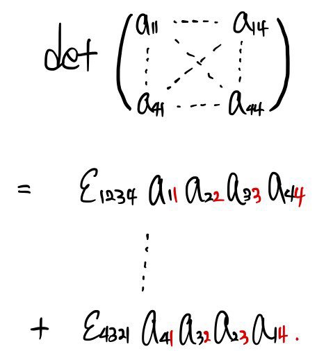
First I’ll write it out like this. Then for the epsilon symbols,

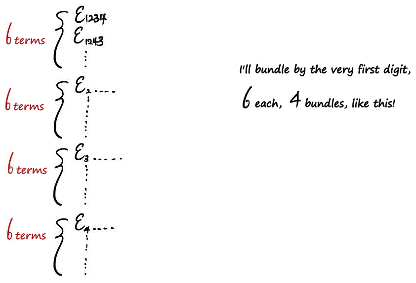
I’m going to sort them by the very first index of the epsilon and bundle them into 4 groups like this.

Why?

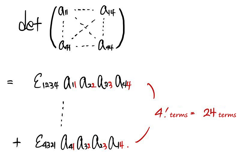
Because I want to bundle this long row of additions into 4 groups. After I’ve bundled them into 4 groups,

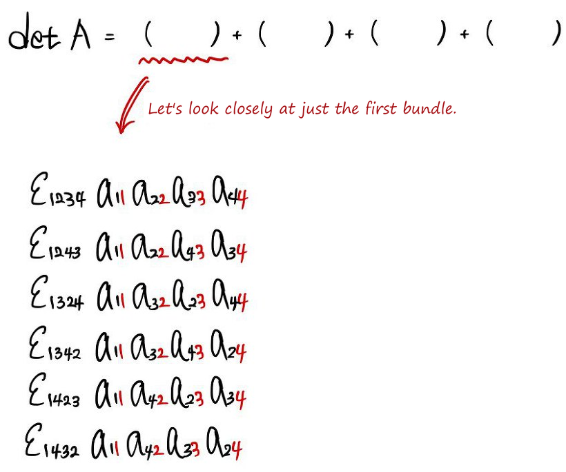
I’m going to figure out the signs of the epsilons in that very first bundle,

and use the fact that the leading index is fixed to do something a little clever (read: a little sneaky). The trick I’m talking about: if something is written as 1234,

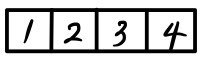
instead of seeing it written like that, we see it as

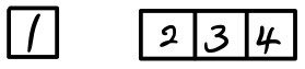
with the split off.

So is

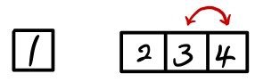
one swap, so “−1”. And is

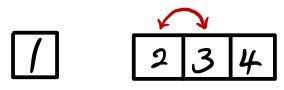
one swap, so “−1”. And so on~~~~.

What I’m saying is~~~~ the split-off 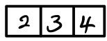doesn’t have to be read as 2, 3, 4 anymore — we can read it as . That’s the move.

And if you look at it that way, it becomes a 3x3 — something we can handle by hand!!!

Because we can think of it like this!!!

(Here $i, j, k$ are 2, 3, 4 in some order, and on the right side they get read as 1, 2, 3.)

That handled the bundle where 1 sits at the front. For the bundle where 2 is at the front, the bundle where 3 is at the front, the bundle where 4 is at the front — same exact principle, they look like this:

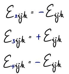
And what we just did here is

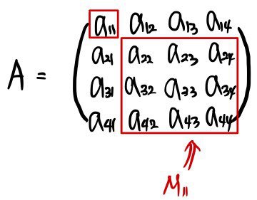
The bundle in the epsilon with 1 at the very front is the bundle that goes with $a_{11}$, and $M_{11}$ is

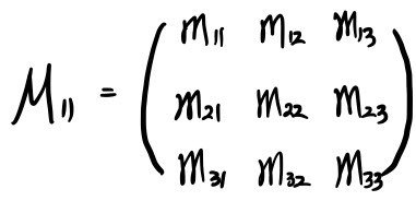
after writing it out again like this,

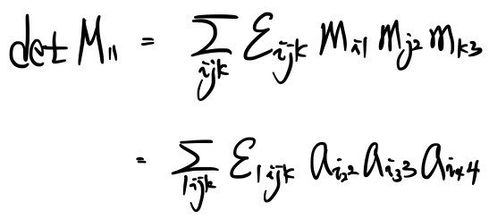
it can be written like this!!!!!

That is — “the first bundle” can be written as . That’s what it means!

Quick one-line summary about capital $M$ before moving on.

Example)

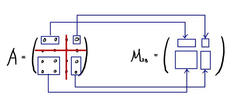
OK so,

first bundle is done. Now think about the second bundle — the epsilon was

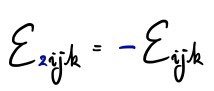
so, . Conclusion:

Any column — and any row

Now, the expression above was built by grabbing the elements $a_{11}, a_{21}, a_{31}, a_{41}$ from column 1 — the first column — and bundling them, right? But the bundling works no matter which column you pull from, one element at a time. In other words,

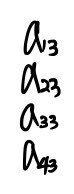
pulling them out one at a time like this, and for each one pulling out its corresponding submatrix, multiplying by the submatrix’s determinant and the sign $(-1)^{k+j}$ (for the entry in row $k$, column $j$), and summing it all up with a sigma — that works too!!!!!

Why does it work for any column though?!?!

Instead of bundling by which value sits at the front of the epsilon (1, 2, 3, or 4), we’d be bundling by which value sits at the 3rd position of the epsilon, right?!? So sure, the epsilon signs might shift around~~~~ — let’s just hand-wave that for now.

(Lucky for us, pulling from column 1 and pulling from column 3 give the same signs, lol)

That is to say,

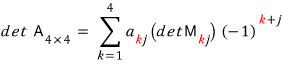
so earlier the discussion fixed $j=1$, but $j$ can be 1, 2, 3, or 4 — doesn’t matter.

But!!!! In the very last post, 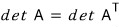we studied this property.

OK OK OK, so the determinant calculation — we took elements from column 1 (the row-1 entry, row-2, row-3, row-4), bundled, and computed — and since the transpose doesn’t change the determinant, we can also take from row 1 (the column-1 entry, column-2, column-3, column-4), multiply each by the determinant of its submatrix (with the sign $(-1)^{i+k}$ for the entry in row $i$, column $k$), and sum them up. Totally fine.

<Imagine doing a Transpose first and then applying the same method as before.> <What had been “pulling row entries out of a column” — once you transpose first to apply the same trick — becomes “pulling column entries out of a row.”>

Example)

An actual 4x4

Let’s stop doing this with letters and try an actual 4x4!!!! That way you’ll really feel what we just did up there!!!

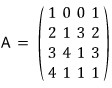
Let’s find the determinant of this matrix!!! Using the method from above!!!

That’s how we said we’d find it, right? So the unpacking goes:

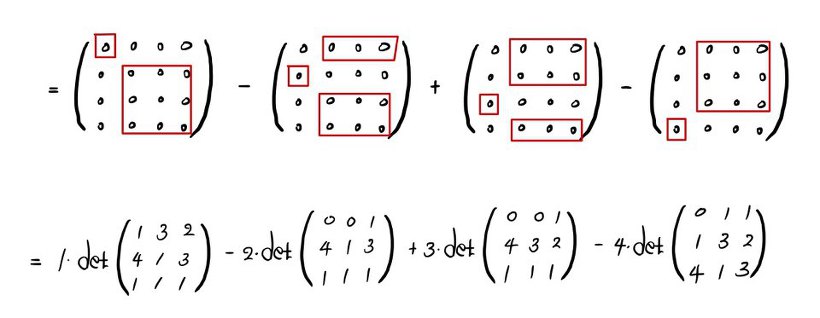
OK so — probably a good moment to point this out: When you find the determinant of a 3x3, you also take the column-1, column-2, column-3 entries of some row, and multiply each pulled entry by the determinant of its corresponding submatrix and add/subtract, right?

Wait. Isn’t that… the cross product calculation?!

In other words, when you try to calculate the 3x3 determinant by the principle above, it turns out to look exactly like the cross product calculation — which is why the cross product is usually written as a 3x3 determinant (with the unit vectors in the top row).

(The cross product itself we’ll revisit later!!!! Don’t sweat the connection yet — catch it when we get there. For now I’ll just leave it at this and move on.) (For the sake of mental health.)

But — when finding the determinant of matrix $A$ above, compared to expanding along column 1 like we just did,

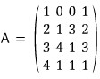
apparently we should know how to see that expanding along row 1 is way more advantageous. The reason it’s easier is super simple: “there are tons of zeros.” Because there are tons of zeros,

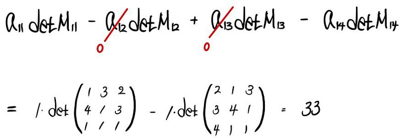
like this, the calculation collapses significantly, and we get our determinant value way faster.

Manufacturing zeros

Hey, you know what????? Human desire knows no bounds, lol lol.

“Isn’t there a way to make this even easier?”

There is. For that, let me copy-paste something from a previous post.

<Copy-paste begins> And let me mention another property of Al.

“The Al value of a matrix where you’ve added a constant multiple of one column to another column is the same as the Al value before you added.”

Totally obvious, right????? (What if you don’t think it’s obvious….. ) Hmm,,,

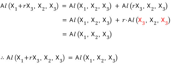
Got it?!?! This pulls some weight later….. you’ll bump into it in the determinant.

<Copy-paste ends> Lol lol lol — and we’re literally bumping into it right now in the determinant. So in the matrix above,

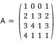
I’ll replace column 1 by column 1 minus column 4.

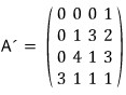
Oh ho~~~~ so then

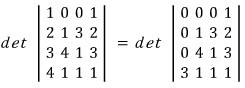
that’s what it means. You caught why I did that operation, right?!?!

It means: by manufacturing a column or row with as many zeros as we can like this before we expand, the calculation gets so much easier!!!

5x5 isn’t scary anymore

Hey, 5x5 matrices aren’t scary anymore!!!

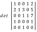
This was terrifying a minute ago, wasn’t it? lol lol lol Let’s pick row 5. Only one nonzero — everything else is 0.

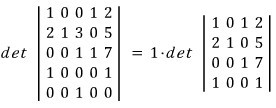
Oh ho~~ now it’s reduced to a 4x4 determinant. Here, let’s pick column 2. Three zeros in column 2.

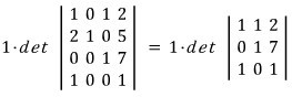
From here on it hardly matters which one we pick (no row or column has more than one zero). What should we go with????? Let’s just pick column 1.

If we’d picked column 2,

Conclusion: no matter how huge the square matrix, as long as you’ve got enough paper and ink, the determinant can absolutely!!!! be found.

Tip: what era are we in, who’s calculating this by hand one entry at a time — is this the Stone Age? I did it in Matlab myself, and in about 5 seconds the answer 6 popped out. lol lol lol

<Screenshot>

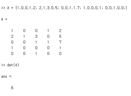
Kidding… heh. The professor said these days no one finds determinants by hand, but there’s a difference between knowing the principle and not knowing it, so he recommended doing it by hand at least once.

---

Heads-up. The figures here are the original notes, slips and all. A few things to watch for:

• In the column-1 expansion of $A$, two entries of the small matrices are miswritten: the third one should be $\begin{pmatrix}0&0&1\1&3&2\1&1&1\end{pmatrix}$ (rows 1, 2, 4 of $A$; the picture has a 4 where the 1 is) and the fourth $\begin{pmatrix}0&0&1\1&3&2\4&1&3\end{pmatrix}$ (the picture has a 1 in row 1, column 2). The values that follow, $1, 3, -2, -11$ and $\det A = 33$, are right.
• The picture labelled "1st-row expansion" shows the formula for a general row $i$, $\sum_k a_{ik}(\det M_{ik})(-1)^{i+k}$; row 1 is the case $i = 1$.