The First Decomposition Theorem
We revisit diagonalization up close — eigenvalues, kernels, and how a 2D space splits into two 1D invariant subspaces — as a warm-up for the full Decomposition Theorem.
Starting with this post, I’m going to dig into block decomposition and diagonalization way more carefully.
We’re going to look at the Decomposition Theorem more, more, more, more carefully than before.
That’s the whole reason we learned polynomials using integers as our toolkit.
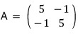
So — that matrix from last time:
I want to describe this thing in slightly different language, and in more detail.
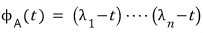
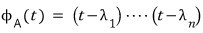
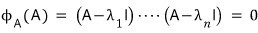
Walking through the diagonalization, we get the characteristic polynomial

.

The roots of this characteristic polynomial are 4 and 6, so the eigenvalues of the matrix are 4 and 6,
and plugging each one into

we hunt down the vectors

that satisfy
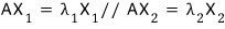
.
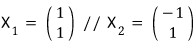
We found them one by one and called them eigenvectors!!!!
And then —
we stack

neatly side by side to build
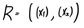
like this, and

by sandwiching A between $R^{-1}$ and $R$ like that, we managed to diagonalize A.
The whole principle

is baked into this.
So then —

we applied this to A and got A'.
And the upshot was: A’ is just A expressed in a different basis… that was the whole story from waaaay back.
OK, let’s revisit what those formulas are actually saying.
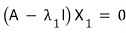
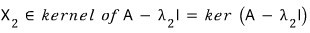
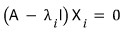
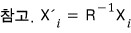
Look at this formula. The vector $X_1$ is a solution of this equation,
and since the right-hand side is zero — it’s a homogeneous equation —
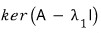
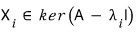
we can also say $X_1$ lives in the kernel of the matrix

.
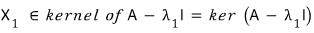
Same deal for $X_2$.
The dimension of each of these kernels turns out to be 1 (I’ll skip the proof here).
So $X_1$ and $X_2$ each span their entire respective kernel all by themselves.
And so —
taking

as a basis for the 2-dimensional space,
we built a new matrix

like this!!!!
(The linear map represented by A takes the form A’ when written in a different basis~~~~)
So if you stare at that formula
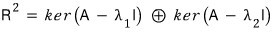
for a sec, it’s also saying that the 2-dimensional space splits into two separate 1-dimensional spaces.
Splitting it like this —
a vector that lives inside
stays inside

no matter how many times you hit it with A,
and the same is true for the subscript-2 one.
This kind of thing shows up in the general diagonalization / block decomposition story.
Which is to say — diagonalization and block decomposition are basically about ‘decomposing’ some vector space…
I’m not totally sure what that means yet, but it sure sounds related to ‘decomposition.’
OK, now let’s look at diagonalization in more general, hairier cases.
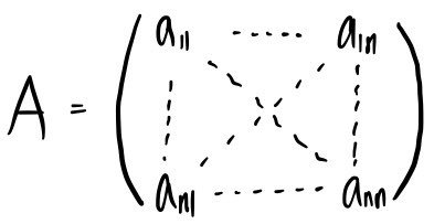
Suppose we have an $n \times n$ matrix like this, with a characteristic polynomial —
※ Note the assumption ※
Assume the characteristic polynomial factors completely into linear factors.
In this setup, we said before that ‘diagonalization is always possible.’
Hmm OK then —
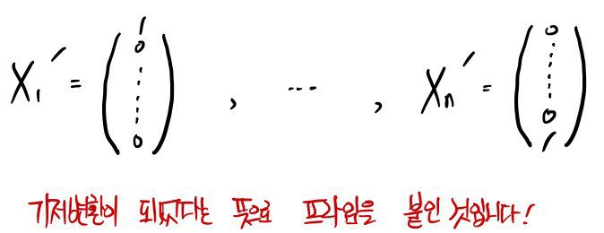
we’ll find $n$ vectors

satisfying
.
We already know each

satisfies
right?!?!?!
And (since diagonalization works) we go grab all $n$ of the

and bundle them up into a matrix R.
Well… R is invertible (we proved this earlier too)
so that means

these are $n$ linearly independent vectors, which means they form a basis!!!!
So if you’ve got any vector Y in the $n$-dimensional space,
it can be written as a linear combination of the $n$

like this:

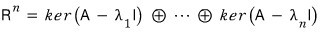
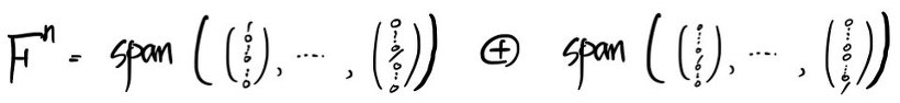
Which is to say —
the $n$-dimensional space

decomposes into the $n$

!!!!

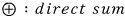
The reason we deliberately throw the direct sum symbol in here —

is because the vectors of the space can be built from a linear combination of vectors in those pieces, and —
we want to emphasize that the way of doing it is unique.
What I mean by that —
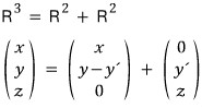
the way of writing $(x, y, z)$ over here is not unique, right?!?!?!
That’s why this one gets written without the direct sum, just a plain old +.
That said — it’s not like you have to use the direct sum every time uniqueness happens,
but it’s nice to use when you specifically want to flag uniqueness.
Anyway, taking A’ as the diagonal matrix and writing it again in
a new basis, we get this!!!!!
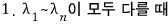
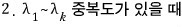
OK now let’s think about the case where the characteristic polynomial doesn’t factor cleanly into distinct linear terms — instead it has ‘multiplicity.’
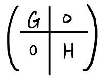
In this setup, by the same principle as before, A’ would look like this:
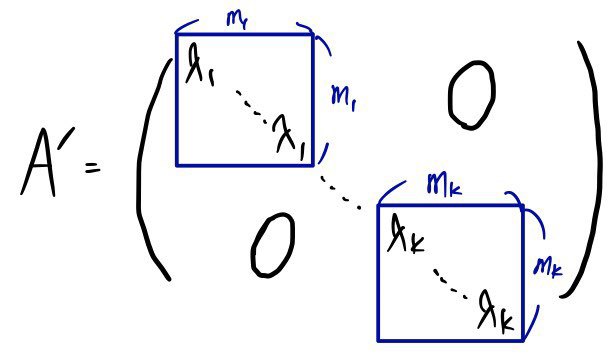
It’s got this structure where small square diagonal blocks line up to form one big diagonal matrix!!!!
If we split the $n$-dimensional space according to the eigenvalues of those diagonal blocks —
splitting everything by eigenvalue —

and over here

— well, that’s how I should put it.
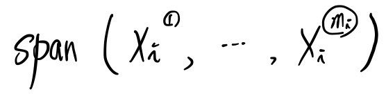
We can write it as a span like this.
Hmm~~~~ you may have forgotten this part.
An eigenvalue can pull in a number of eigenvectors equal to its own multiplicity!!!
So —

this thing is also called an eigenspace.
The dimension of each one is

.
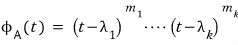
Let me organize this one more time, with a slightly different reading.
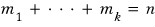
In this case the characteristic polynomial is
like this,
and when we diagonalize, the $n$-dimensional space gets split into
$n$ spaces like that.
cf.) By Cayley-Hamilton, what happens if we plug A itself in for $t$?!?!?!
It became zero, right.
we got this, right.
Wait — but the matrices in those kernels and the matrices we’re multiplying in Cayley-Hamilton are the same thing!!!
To say it again: if there’s a polynomial that becomes 0 when you plug A in for $t$, that polynomial is showing you how the $n$-dimensional space decomposes.
Can’t we say that????????????????????????????????????????????????????
We’ll come back to this later.
For this case, let’s now write the polynomial
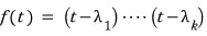
like this.
Since it’s the characteristic polynomial with all the multiplicities stripped off, it’s a different polynomial — that’s why I wrote it as $f(t)$.
Going back to how we split everything into eigenspaces —
the $n$-dimensional space gets split into
$k$ spaces like that,
and if we plug A into $f(t)$, then $f(A) = $….. 0.
(Since it’s just the characteristic polynomial with the exponents (multiplicities) stripped, I think you can buy that it still hits 0 without much trouble.)
In other words — if a polynomial evaluated at A gives the zero matrix,
then the way $f(t)$ factors is what determines the ‘decomposition’ of the $n$-dimensional space.
Remember earlier when we defined that set called
$I_{A}$
?
It was the set of all polynomials that hit 0 when you plug A in for the variable.

So — the decomposition of A is determined by the factorization of $f(t)$!!!!!!!!!!
Reading this, a question probably popped up in your head:
“Hey (annoyed face) — what if there’s a term that doesn’t factor into linear pieces?”
(Like, what are you going to do if you’ve got something like

sitting there?)
OK — that’s where we have to start talking about the “First Decomposition Theorem.”
Let me spoil the First Decomposition Theorem real quick and then prove it.
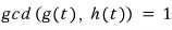
And if
($\gcd(g(t), h(t))$ just means $g(t)$ and $h(t)$ share no common divisor other than 1. The two are ‘coprime’ — no common factor!!!!)
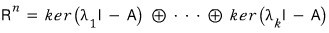
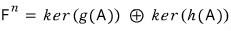
then the $n$-dimensional space decomposes into kernels like
— and that’s the ‘First Decomposition Theorem.’
When you have a matrix like this, picking an appropriate basis
turns it into this — that’s the claim.
It splits like this…. spoiler over.
Now let me prove it.
$f(A) = 0$. $g(t)h(t)$ are coprime.
If $g(t)$ and $h(t)$ are coprime,
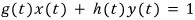
then there exist $x(t), y(t)$ satisfying
!!!!!!
(Take a peek at the earlier post. It’s the same statement as: if integers $a, b$ are coprime then there exist $x, y$ with $ax + by = 1$.)
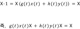
Take any vector X in the $n$-dimensional space, multiply it by 1, and write that ‘1’ all dramatically:

now plug A in for $t$.

Written this way — since $f(A) = g(A)h(A) = 0$,
the red vector out front is a vector that gets killed when you multiply by $h(A)$,
and the blue vector behind is a vector that gets killed when you multiply by $g(A)$!!!!
So — the front one dies under $h(A)$, meaning it lives in $\ker(h(A))$,
and the back one dies under $g(A)$, meaning it lives in $\ker(g(A))$.
Therefore,
And the reason we deliberately wrote direct sum is to emphasize the result is uniquely determined.
Since they’re coprime, $x(t), y(t)$ are uniquely pinned down…..
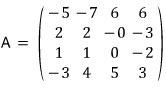
Let’s run an actual example to see whether this First Decomposition Theorem still works for matrices that can’t be diagonalized.
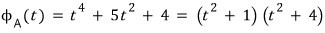
For this matrix A, let’s find an $f(t)$ with $f(A) = 0$.
We can just use the characteristic polynomial — easiest path — so let’s go that route.
(Over the real numbers) you can’t factor it any further.
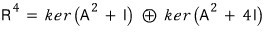
OK so now let’s follow the First Decomposition Theorem.
This formula is supposed to hold, so let’s check it.
Since
,
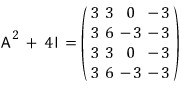
it works out like this.
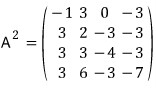
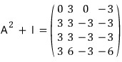
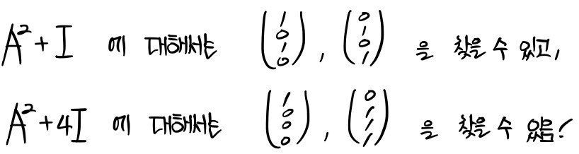
To think about each kernel, let’s hunt down the vectors that get killed when you hit them with these on the right.
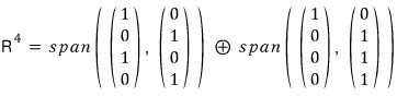
They’re linearly independent!~ Confirmed — now let’s span.

Just like in diagonalization, we gather those vectors into R,
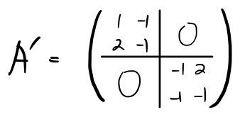
and when we apply it to A like this

we can confirm it does in fact end up like that.
The power of block decomposition: as you saw above, a quest in 4-dimensional space gets reduced to two 2-dimensional ones — that’s the whole pitch!!!!!!!
Originally written in Korean on my Naver blog (2016-01). Translated to English for gdpark.blog.
Comments
Discussion happens via GitHub Discussions. You'll need a GitHub account to comment.