Logistic Regression Part 3

Alright, like I mentioned last time — today we’re looking at multi-class classification.

Everything we’ve done so far? The data was always split into two buckets. 0 or 1. Binary. Done.

But what if we’ve got 3 or more classes to sort out? How do we bend our current classifier to handle that?

So how do you classify 3+ things?

Right now we’ve got a classifier that can separate two things. The question is: can we cheat our way into using it for three?

Let’s look at a picture.

OK so the points are clustered by color. With just our binary classifier, we can already do this much:

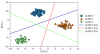
• A blue line separating blue from everything else
• A green line separating green from everything else
• A red line separating red from everything else

That’s all doable with what we already have.

Wait a sec…

If we’ve got that much, can’t we pull off 3-class classification with some sneaky trick? What kind of dirty trick should we try here?!

Here’s what I’m thinking.

First, the broad regions — the areas where each color obviously clumps up — those are easy. Just use the “above or below the line” rule for each of the three lines. Done.

The tricky bit is the triangle in the middle where all three lines meet. For every point inside that triangle, measure its distance to all 3 lines.

Then for each point:

• “Oh, point 1 — you’re closest to blue → you’re blue.”
• “Oh, point 2 — you’re closest to red → you’re red.”
• “Oh, point 3 — closest to blue → blue.”
• “Oh, point 4 — closest to blue → blue.”
• “Oh, point 5 — closest to green → green.”

Do that for every point and you get something like:

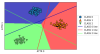
So yeah — the thing I just described is literally an algorithm called one-vs-rest (OvR).

But lol, there are only like 5 points here. What if the dataset gets huge? Measuring distance from every point to every line would take forever. At some point you just GG and back out.

Anyway — let’s eyeball it and move on.

Because our goal right now isn’t to understand every single internal of every ML algorithm, right? Our goal is to use this stuff!

The parameter

Super simple. There’s a parameter called multi_class, and for the one-vs-rest method we just covered, you write:

multi_class='ovr'

Let’s get it!

First, load the data:

from sklearn.datasets import load_iris
iris = load_iris()
X = iris['data']
y = iris['target']

Shuffle & split:

from sklearn.model_selection import train_test_split
X_train, X_test, y_train, y_test = train_test_split(X, y, random_state=1, stratify=y)

The iris dataset is 3-class and the class ratios are nicely balanced:

import pandas as pd
X = pd.DataFrame(X)
y = pd.Series(y)
print(y.value_counts()/len(y))

2    0.333333
1    0.333333
0    0.333333
dtype: float64

Now let’s fit with multi_class='ovr' and see what we get. I’ll just throw in the other parameters at reasonable values:

from sklearn.linear_model import LogisticRegression
model = LogisticRegression(C=1, 
                           class_weight='balanced', 
                           random_state=1, 
                           multi_class='ovr', 
                           n_jobs=-1, 
                           solver='lbfgs').fit(X_train, y_train)

print('train score: ', model.score(X_train, y_train))
print('test score:  ', model.score(X_test, y_test))

train score:  0.9285714285714286
test score:   0.9210526315789473

“But wait, is it really predicting all 3 classes correctly??”

Fine, let’s check. I’ll dump both train and test sets through predict at once:

print('predictions: ', model.predict(X))

predictions:  [0 0 0 0 0 0 0 0 0 0 0 0 0 0 0 0 0 0 0 0 0 0 0 0 0 0 0 0 0 0 0 0 0 0 0 0 0 0 0 0 0 0 0 0 0 0 0 0 0 0 2 1 2 1 1 1 2 1 1 1 1 1 1 1 1 1 1 1 1 1 2 1 1 1 1 1 1 2 1 1 1 1 1 1 1 1 2 1 1 1 1 1 1 1 1 1 1 1 1 1 2 2 2 2 2 2 1 2 2 2 2 2 2 1 2 2 2 2 2 1 2 2 2 2 2 2 2 2 2 2 2 2 2 1 1 2 2 2 2 2 2 2 2 2 2 2 2 2 2 2]

There it is — it’s predicting 0, 1, and 2. All three classes.

And we can look at how confident each prediction was like this:

print('predict_proba: ', model.predict_proba(X))

Hey — we learned precision and recall too, so let’s use those!

Heart’s pounding a bit lol — will it actually give us precision and recall for each of the 3 classes separately…? heh heh heh

from sklearn.metrics import classification_report
pred_train = model.predict(X_train)
pred_test  = model.predict(X_test)
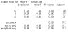
print('classification_report - train')
print(classification_report(y_train, pred_train))

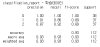
Ohhhhhh

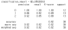
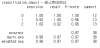
print('classification_report - test')
print(classification_report(y_test, pred_test))

Besides OvR — there’s also multinomial

model = LogisticRegression(C=1, class_weight='balanced', random_state=1, multi_class='multinomial', n_jobs=-1, solver='lbfgs').fit(X_train, y_train)
print('train score: ', model.score(X_train, y_train))
print('test score:  ', model.score(X_test, y_test))

train score:  0.9642857142857143
test score:   0.9736842105263158

pred_train = model.predict(X_train)
pred_test  = model.predict(X_test)
print('classification_report - train')
print(classification_report(y_train, pred_train))

print('classification_report - test')
print(classification_report(y_test, pred_test))

The numbers came out a little nicer, heh heh heh.

Apparently multinomial is generally better because it uses a softmax-based approach under the hood. As for what softmax actually is — we’ll get to that when we briefly touch Deep Learning later. So I’m shelving that concept for next time, heh heh.

OK — we’re not gonna stop at just “hey we classified 3 things.” Let’s keep moving.

Up next…

SVM!

Originally written in Korean on my Naver blog (2019-11). Translated to English for gdpark.blog.