Goods Market and the Short-Term Model

OK so up until now everything I’ve been calling “economics” was really liberal-arts-flavored economics — and now, finally, the actual major-level stuff is starting.

Gonna try to chip away at it, slow and steady.

For the content side, I’m rolling with Blanchard’s macro textbook~

Jumping in from Chapter 3. The Goods Market. (Anything before that is too much “background knowledge” for us to be spending time on…)

First — composition of GDP.

C + I + G + NX

The thing to watch for: the investment piece here is not inventory investment, it’s fixed investment (residential + non-residential).

Then what’s inventory investment?

Literally — think of it as the cost spent to keep your leftover stock sitting nicely on the shelf.

• Production − Sales = Inventory Investment

This holds, so

Production = Sales + Inventory Investment

Which means inventory investment is NOT part of production!!!

And one more bit of common-sense bookkeeping:

G does not capture all ’transfer expenditures.'

(Health insurance, social security payouts, interest payments on the national debt, that kind of stuff.)

And so —

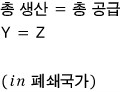
※ Assumption alert ※: closed economy.

Total demand inside a closed economy can be written as C + I + G.

(I just called GDP “total demand” — that’s fine, right??? “Three-sided equivalence of national income”: equilibrium total production = equilibrium total expenditure = equilibrium total income.)

Now we’re gonna take each of these guys apart and stare at them one by one.

Why? Because we want to nail down: “what variable is each one actually a function of???”

① C (Consumption)

Obviously, what people consume gets pushed around by a huge number of variables,

but the one taking the biggest slice is, at the end of the day, income.

Not just income, though.

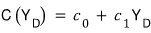
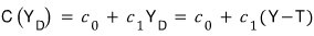
You can simplify and say it’s disposable income — the money left after paying all~~~ your taxes — that drives consumption behavior.

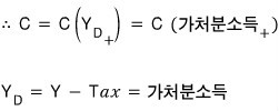
And the meaning of that little (+) subscript is:

if this ↑,

then the function value is ↑ too — that’s the (+) positive relationship.

When I first ran into this notation I was like, why on earth would you write it this way,

but unlike the physics I’m used to, econ seems to be pretty cautious with the word ‘proportional.’

In society, basically nothing is exactly proportional,

so it’s apparently more correct to say “in a positive relationship” than to drop the strong word ‘proportional’ on it.

From here on I’ll use this subscript trick to mark whether each independent variable is positive or negative.

OK, and now another assumption sneaks in.

※ Assumption alert ※

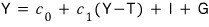
Let’s say the C function and disposable income have a first-order linear relationship.

Now we can write it down with confidence.

Like this —

and the two constants c0, c1 mean:

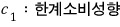
If a person’s disposable income goes up by one unit, how much more do they consume?

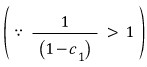
Then c1 has to be less than 1.

Because nobody — well, OK, almost nobody — earns an extra 10,000 won and then somehow spends 15,000 won more than before!!!

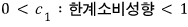
(This is the MPC you saw back in micro — remember??)

And this thing —

we can call the ‘marginal propensity to save,’ right?

Whatever you don’t consume, you save. (You’ll use it later ^^)

Then what about c0??

c0 is what you’d consume when disposable income is 0 — so does that mean c0 should be zero too?!?!

Nah nah, no way! Even when people aren’t pulling in any money, they still need to eat to live.

So consumption is always there, and……

c0, apparently, is like an ‘overdraft account.’ (negative saving)

Alright, so consumption is:

② Now the government-side variables G and T.

G and T should be treated as exogenous variables (independent variables not explained inside the model)!!!

Or — well, let’s just assume they are!!!

The reason this assumption is reasonable is

that the government’s decision-making process is just different from a consumer’s or a firm’s!!!!

Like, no — there’s no way the reasoning behind a government choice should look the same as the reasoning behind a consumer’s or a firm’s choice!!!

Right, think about why the state exists in the first place… that kind of thinking…… (the sort of “stuff private firms won’t do, the state has to do” line of thought… heh)

Alright, and the more fundamental reason it has to be treated as exogenous is

that a macroeconomist’s whole goal is: with respect to the independent variables G & T, how do all the other variables move~~~~~

That’s what we want to see.

Which is exactly why, in our model, G and T get to sit in the “independent variable” seat.

And we still need to look at the third piece, investment (I), but…

we’ll deal with that later. It’ll show up when we start talking about interest rates.

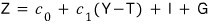
OK — so now we know the whole of total demand (Z). (Let’s call it Z..? That’s fine, right? haha)

This is total demand from an aggregate-level view, swinging around with whatever variables people are reacting to.

“We can pin down the range of Z values that are possible given the domain of the variables.” That’s the kind of statement we’re making here,

and from this point, the question pops up:

“I want total demand at exactly this one specific moment in time!”

Answer: “If you know the values of every variable at that moment, sure, you can know it.”

But… that’s basically out of the question.

So we have to phrase it differently:

At any given point in time, in each respective moment,

total demand and total supply (production) will be sitting at the same scale.

They’ll somehow be in equilibrium.

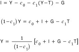
That is,

Now I’m gonna mess around with this equation.

Since this is an equation about the ’equilibrium point,’

we can say it’s an equation about ’equilibrium output,’ right?^^*

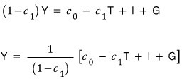
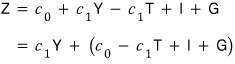
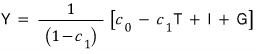
I’m gonna rewrite this Y like so and then read off what it’s saying.

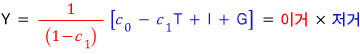
The reason I split it up like this….

you’ll see in a sec.

*that (in blue):

The blue ’that’ terms — at the very least — are not functions of Y!!!!!

They’re called autonomous spending, because what they’re saying is: however much production happens, the values of these terms don’t budge!!!

So the point is, consumption going up by +1 doesn’t automatically mean production goes up by +1!!!

*this (in red):

And it’s not the case that if autonomous spending changes by +1, Y also changes by +1 right alongside it —

instead, Y changes by the change in autonomous spending

multiplied by

It changes by more than the change in autonomous spending!!!!

So “this (in red)” —

this guy is what we call the multiplier!!!

Alright, what this is really saying is that Y moves beyond the direct hit from autonomous spending,

and to put it in everyday terms:

income rises → demand goes up → so production rises → so income rises again → demand goes up again → ·······

Like that —

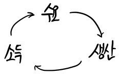
that whole philosophy is baked in here…

Now I’m gonna take everything we’ve done and

redraw it as a graph,

and pull out the final conclusion.

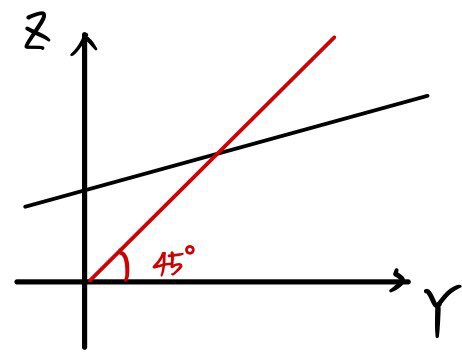
Let’s try to remember

this thing from 8th-grade math.

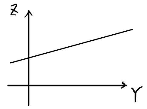
Then the graph above reads as a first-degree line drawn with slope c1 and y-intercept c0 − c1T + I + G!!!

Thing to watch: the slope has to be drawn as less than 1!!!!

Because c1 — the slope — is, no matter what, somewhere between 0 and 1!!!

And the corresponding Z value equals the Y value at that point.

That is, equilibrium at Z = Y!!!!!!

So that’s why~~!!

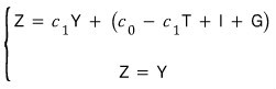
The solution of this system is exactly the equilibrium demand and equilibrium output we derived above.

Y = Z

I don’t need to explain how to draw this, right?

You sketch it like that and you’re done~

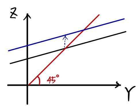
Now, in the middle of all this,

suppose,

the autonomous spending part — i.e. the y-intercept — suddenly goes pop!~ and jumps up.

Then the rise should be exactly the length of that arrow, but in fact Z doesn’t settle into equilibrium at that exact amount —

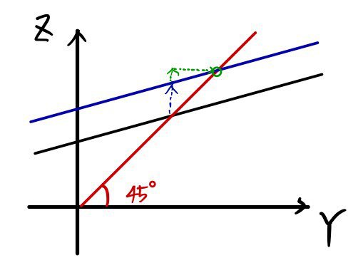
it lands at a slightly~~ higher point, doesn’t it?!?!?!

Comparing before and after the y-intercept jump, it doesn’t rise 1-to-1 —

the multiplier effect is layered on top.

That’s it!!! heh heh heh

That’s the multiplier effect, drawn out in a graph!!

3 little pictures resolve everything we just said in words above. heh heh heh

cf.)

or

The field that tries to actually go out and find these coefficients… these functions… is called “econometrics.”

(Sounds like it would be ridiculously interesting… seriously… heh)

cf.) Wait wait wait wait — “those kinds of changes — how much time do they take?”

So far, we’ve been saying production is always equal to demand, so when demand changes,

production changes immediately (instantly)~

That’s basically what we’ve been claiming.

Honestly — this makes zero sense by common-sense standards.

Because in reality there’s obviously a time lag!!!! (And the kinds of time lags are also wildly varied, and yeah it takes an insane amount of time!)

To patch this, economists apparently try to close the gap with reality through a thing called “adjustment dynamics.”

But dealing with that is too much for us right now, so we’ll skip it.

(Just keep the sense that something like this exists~?)

Alright, so up to here we’ve finished looking at equilibrium in the goods market from the perspective of —

Same content as above, but apparently there’s a ‘different angle’ we can look at it from.

Let’s grab that and move on.

That angle is: viewing this through investment and saving.

We humans, from our income, after paying all~~ the taxes, are left with disposable income,

we spend whatever we want to spend on consumption, and the leftover money — that all~~ gets saved.

Can we say that?!?

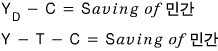
Therefore,

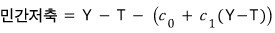
(Embedded assumption: same as we did above with the consumption function — disposable income and this thing have a first-order linear relationship.)

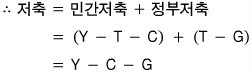
But — there’s one more entity that can save.

The government can also save.

Picture it: [the government] collects all the money via taxes, spends some of it on government expenditures,

and whatever’s left over, saves.

(That B in parentheses — strictly we’d also have to think about whether bonds were issued for the sake of government saving.

But the goal right now is just understanding, so let’s say ΔB = 0 — the amount of government bonds outstanding hasn’t changed.)

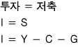
And by the same logic as before — “how much investment will there be??”

→

“Whatever it works out to, investment and saving will be equal!! Because that’s the equilibrium!!!”

Now into C, I’ll plug in the consumption equation — er, the consumption-behavior equation — we used above.

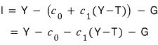
So apparently the same equation we got above can also be derived this way!!!! kyakyakyakya

Annnd — we just revealed the relationship between I and S, didn’t we????

This is what’s called the IS relationship.

What I and S revealed was the ‘goods market’ itself, right?

So when we say “IS relationship,” we can think of it as just “the goods market.”

Later on we’ll derive the IS curve.

When we get there, just go: “ah, this guy’s about to draw the curve of the goods market.” heh heh heh

And like that — once we’ve simply modeled aggregate supply Y and aggregate demand Z in the goods market, the macro analysis is done.

Following this little model, can we actually pin down G and T and predict / steer the world’s demand and supply???

NONONONONONONONONO!!!!!! This model is way too simple, and the gap with reality is apparently enormous.

For starters:

1. Actually changing G and T is supposedly not an easy thing. You hit difficulties before you even pass the legislation….

2. I derived I by treating it as a fixed constant, but honestly that’s wrong — the things that could shift I are endless.

3. The closed-economy assumption, this is basically a story from some other planet. (Even North Korea isn’t a fully sealed-off economy……. heh heh heh)

4. People’s expectations have a ridiculous amount of pull.

5. The fact that, if asked, you could rattle off 500 more reasons too obvious to bother writing down.

Ugh….. (crying) so why did we do all of this??? Have we been doing something pointless? (crying)

Apparently — no, that’s not quite right either.

Because those variables we assumed to be constant —

from “a sufficiently short short-term perspective” — really can be treated as constant, they say.

And that’s exactly why we can call it a short-term model,

so this model is called a short-term model!!!! heh

Originally written in Korean on my Naver blog (2016-01). Translated to English for gdpark.blog.